1. Pi0.5 整体架构
Pi0.5 是一个基于 Flow Matching 的 VLA(Vision-Language-Action)模型。它的核心思路是:用 PaliGemma(SigLIP + Gemma)编码图像和语言指令,用单独的 Action Expert(另一个小 Gemma)去噪生成动作序列。
1
2
3
4
5
6
7
8
9
10
11
12
13
14
15
16
17
18
19
20
21
22
23
24
25
26
27
28
| ┌─────────────────────────────────┐
│ PI05Policy │
│ (PreTrainedPolicy ) │
│ │
│ ┌───────────────────────────┐ │
│ │ PI05Pytorch (model) │ │
│ │ │ │
│ │ ┌─────────────────────┐ │ │
│ │ │ PaliGemmaWithExpert │ │ │
│ │ │ │ │ │
│ │ │ paligemma (VLM) │ │ │
│ │ │ ├─ vision_tower │ │ │
│ │ │ │ (SigLIP) │ │ │
│ │ │ └─ language_model │ │ │
│ │ │ (Gemma 2B/300M) │ │ │
│ │ │ │ │ │
│ │ │ gemma_expert │ │ │
│ │ │ (Gemma 300M/2B) │ │ │
│ │ └─────────────────────┘ │ │
│ │ │ │
│ │ action_in_proj (Linear) │ │
│ │ action_out_proj (Linear) │ │
│ │ time_mlp_in/out (MLP) │ │
│ └───────────────────────────┘ │
│ │
│ rtc_processor (RTCProcessor) │
│ _action_queue (deque) │
└─────────────────────────────────┘
|
1.1. 关键组件关系
| 组件 |
文件 |
职责 |
PI05Config |
configuration_pi05.py |
超参数:chunk_size=50, max_action_dim=32, flow matching 参数 |
PaliGemmaWithExpertModel |
modeling_pi05.py:328 |
核心 NN:PaliGemma VLM + Action Expert Gemma 的联合推理 |
PI05Pytorch |
modeling_pi05.py:534 |
训练/推理逻辑:flow matching 的 forward 和 sample_actions |
PI05Policy |
modeling_pi05.py:898 |
LeRobot 适配层:对接 batch dict ↔ 模型,管理 action queue |
make_pi05_pre_post_processors |
processor_pi05.py |
构建预处理/后处理 pipeline |
RTCProcessor |
rtc/modeling_rtc.py |
Real-Time Chunking:用前一个 chunk 的 leftovers 引导当前去噪 |
2. 从全链路流经PI05模型(源码角度)
数据流分两路:训练 (forward) 和 推理 (select_action)。我逐阶段走一遍。
2.1. 数据准备阶段
2.1.1. LeRobotDataset 输出 → batch dict
数据集加载后,每个 batch 是一个 dict,包含:
1
2
3
4
5
6
7
| batch = {
"observation.images.camera1": Tensor[B, 3, H, W],
"observation.state": Tensor[B, state_dim],
"action": Tensor[B, T, act_dim],
"task": List[str],
"dataset_index": ...
}
|
2.1.2. Pre-Processor Pipeline(训练/推理共用)
由 make_pi05_pre_post_processors() 构建,6 个 step 顺序执行:
1
2
3
4
5
6
7
8
9
10
11
12
13
14
15
16
17
18
19
20
21
22
23
24
25
26
27
28
29
30
31
32
33
| Raw batch dict
│
▼
[1] RenameObservationsProcessorStep — 重命名特征 key(如 left → camera1)
│
▼
[2] AddBatchDimensionProcessorStep — 为每个 feature 加 batch 维度
│
▼
[3] NormalizerProcessorStep — 用数据集 stats 做归一化
│ STATE → QUANTILES 归一化(到 [-1, 1])
│ ACTION → QUANTILES 归一化
│ VISUAL → IDENTITY(原样通过,Pi0.5 自己处理图像归一化)
│
▼
[4] Pi05PrepareStateTokenizerProcessorStep — 关键步骤!
│ ① 将归一化后的 state 离散化为 256 bins(digitize)
│ ② 构造文本 prompt:
│ "Task: {task}, State: 12 34 56 ... 200;\nAction: "
│ ③ 将 prompt 存回 complementary_data["task"]
│
▼
[5] TokenizerProcessorStep — 用 PaliGemma tokenizer 分词
│ prompt → token_ids [B, max_length=200]
│ 生成 attention_mask
│ 输出到 batch["observation.language.tokens"]
│ batch["observation.language.attention_mask"]
│
▼
[6] DeviceProcessorStep — 将所有 tensor 移到 GPU
│
▼
处理后的 batch dict → PI05Policy.forward() / select_action()
|
关键设计点:步骤 [3] 和 [4] 的顺序是强制依赖 — Normalizer 必须先于 Pi05PrepareStateTokenizer,因为 tokenizer 的 discretize 需要 state 已经是 [-1, 1] 范围。
2.2. 训练 Forward Pass
2.2.1. 训练全数据流概览
1
2
3
4
5
6
7
8
9
10
11
12
13
14
15
|
batch dict
│
├─► _preprocess_images(images)
│ ├─ 格式检测:[B,C,H,W] → [B,H,W,C] → resize_with_pad → [B,H,W,C]
│ ├─ Resize with pad: 保持宽高比,黑边填充到 (224, 224)
│ ├─ 归一化 [0,1] → [-1,1](SigLIP 输入格式)
│ ├─ 转回 [B,C,H,W]
│ └─ 缺失相机 → 创建全 -1 dummy image + mask=0
│
├─► tokens = batch["observation.language.tokens"] [B, 200]
├─► masks = batch["observation.language.attention_mask"] [B, 200]
│
└─► prepare_action(batch) → pad_vector(action, max_action_dim=32)
|
然后进入 PI05Pytorch.forward() — Flow Matching 训练核心:
title1
2
3
4
5
6
7
8
9
10
11
12
13
14
15
16
17
18
19
20
21
22
23
24
25
26
27
28
29
30
31
32
33
34
35
36
37
38
39
40
41
42
43
44
45
46
47
48
49
50
51
52
53
54
55
56
57
58
59
60
61
62
63
64
65
66
67
68
69
70
71
72
73
74
75
76
77
78
79
80
81
82
83
| Flow Matching Forward
═══════════
Step 1: 采样噪声和时间
─────────────────────
noise ~ N(0, 1) shape: [B, chunk_size=50, max_action_dim=32]
time ~ Beta(α=1.5, β=1.0), scaled to [0.001, 0.999]
shape: [B]
Step 2: Flow Matching 插值
─────────────────────────
x_t = t * noise + (1-t) * action
u_t = noise - action
Step 3: embed_prefix() — 编码 Prefix(图像+语言+状态)
──────────────────────────────────────────────────
┌──────────────┐ ┌──────────────┐ ┌──────────────────┐
│ Images │ │ Language │ │ State (在 token │
│ [B,3,224,224]│ │ tokens │ │ 中已离散化) │
└──────┬───────┘ └──────┬───────┘ └────────┬─────────┘
│ │ │
▼ ▼ ▼
SigLIP vision Gemma embed_tokens 已嵌入在 language
embed_image() × sqrt(d) tokens 的文本中
│ │
▼ ▼
[B, N_img, 2048] [B, 200, width]
│ │
└────────┬──────────┘
▼
torch.cat → prefix_embs [B, N_img+200, width]
prefix_pad_masks [B, N_img+200]
prefix_att_masks [B, N_img+200] (全是 0,表示 prefix 内部可以互相 attend)
Step 4: embed_suffix() — 编码 Suffix(噪声动作+时间)
──────────────────────────────────────────────────
noisy_actions [B, 50, 32] + timestep [B]
│ │
▼ ▼
action_in_proj Sinusoidal pos
→ [B, 50, width] embedding → [B, width]
│
▼
time_mlp_in → SiLU → time_mlp_out → SiLU
→ adarms_cond [B, width] ← 用于控制 AdaRMS Norm
│
▼
suffix_embs [B, 50, width]
suffix_pad_masks [B, 50] (全 1)
suffix_att_masks [B, 50] (第 0 位=1, 其余=0, 因果注意)
Step 5: 拼接 Prefix + Suffix,构建 Attention Mask
──────────────────────────────────────────────
full_embs = [prefix_embs | suffix_embs] [B, N_prefix+50, width]
att_masks: prefix 全 0(互相可见),suffix 因果
通过 make_att_2d_masks() 构建 2D attention mask:
- prefix token 可以看所有 prefix token
- suffix token 因果看之前的 suffix token + 所有 prefix token
- 转换为 4D mask (OPENPI_ATTENTION_MASK_VALUE = -2.3819763e+38)
Step 6: 联合 Transformer Forward
──────────────────────────────
PaliGemmaWithExpertModel.forward(inputs_embeds=[prefix, suffix])
18 层联合处理,每层:
① PaliGemma 和 Expert 的 hidden states 分别做 input_layernorm (含 adarms_cond)
② QKV 投影后 concat 到一起
③ 联合 self-attention(prefix+suffix 在一起做 attention)
④ 分开做 o_proj → residual → post_attention_layernorm → MLP → residual
⑤ 支持 gradient checkpointing 逐层重计算
Step 7: 输出投影 + 计算 Loss
──────────────────────────
suffix_out = last_hidden_state[:, -50:, :]
suffix_out → action_out_proj → v_t [B, 50, 32]
loss = MSE(u_t, v_t)
截断到真实 action dim(去掉 padding 部分)
|
2.2.2. Flow Matching
1
2
3
4
5
6
7
8
9
10
11
12
13
14
15
16
17
18
19
20
21
|
Step 1: 采样噪声和时间
─────────────────────
noise ~ N(0, 1) shape: [B, chunk_size=50, max_action_dim=32]
time ~ Beta(α=1.5, β=1.0), scaled to [0.001, 0.999]
shape: [B]
Step 2: Flow Matching 插值
─────────────────────────
x_t = t * noise + (1-t) * action
u_t = noise - action
...
Step 7: 输出投影 + 计算 Loss
──────────────────────────
suffix_out = last_hidden_state[:, -50:, :]
suffix_out → action_out_proj → v_t [B, 50, 32]
loss = MSE(u_t, v_t)
截断到真实 action dim(去掉 padding 部分)
|
2.2.2.1. x_t — 插值后的含噪动作
这是一条从干净动作到纯噪声的直线路径:
1
2
3
| t=0 (几乎): x_t = 0·noise + 1·actions = actions ← 干净动作
t=0.5: x_t = 0.5·noise + 0.5·actions ← 各一半
t=1: x_t = 1·noise + 0·actions = noise ← 纯噪声
|
1
2
3
4
5
6
7
8
9
10
11
12
13
| 噪声空间
↑
│ noise ●─────────────────● x_t (t=0.8, 大部分是噪声)
│ \
│ \
│ ● x_t (t=0.5, 一半一半)
│ \
│ \
│ ● x_t (t=0.2, 大部分是干净动作)
│ \
│ actions ●──────────→ 数据空间
│
└──────────────────────────────────────→
|
每个 time 值唯一确定这条线上的一个点。训练时随机采样 t,让模型学习不同噪声水平下的去噪。
对时间进行采样, 例如 B=4 时:
1
2
3
| time = [0.23, 0.87, 0.51, 0.03]
↑ ↑ ↑ ↑
样本0 样本1 样本2 样本3 各自独立,不做排序
|
需要注意的是, 每个样本只采样一个时间来进行训练! 而不是采样整条从(0,1)的时间段
一个 batch 里混合不同噪声水平的样本,模型的梯度和 loss 同时来自轻噪和重噪样本,训练更稳定。如果用同一个 t 给整个 batch,模型在每个 step 只能学会在单一噪声水平下去噪,收敛慢很多。
2.2.2.2. u_t — 速度场目标
这是 Rectified Flow 的关键特性:直线路径的速度场是常数。
1
2
3
| x_t = t·noise + (1-t)·actions
dx_t/dt = noise - actions = u_t ← 恒定速度,不随 t 变化
|
物理直觉:如果你从 actions 出发,以恒定速率 noise - actions 运动,在 t=1 时恰好到达 noise。模型的训练目标就是预测这个恒定速度,即 v_t ≈ u_t。
如果有两条数据在同一个点产生的速度方向不同怎么办?😨
由于使用的是均方差, 可以证明实际上得到的速度是他们的平均, 所以实际上学到的速度场并不是全部都是直线
2.2.2.3. 训练 vs 推理
|
时间方向 |
起点 |
终点 |
公式 |
| 训练 |
t: 0→1 |
actions |
noise |
学习预测 v_t ≈ noise - actions |
| 推理 |
t: 1→0 |
noise |
actions |
逆向积分 x_{t-Δt} = x_t + Δt · v_t |
1
2
3
4
5
6
7
8
9
10
11
|
x_t = t * noise + (1-t) * actions
u_t = noise - actions
loss = MSE(model(x_t, t), u_t)
x_t = noise
for step in range(N):
v_t = model(x_t, t)
x_t = x_t + dt * v_t
|
2.2.3. PaliGemma
2.2.3.1. SigLIP
SigLIP完整前向流程
以一张图 [B, 3, 224, 224] 为例:
Step 1: Patch Embedding(卷积切块)
1
2
3
4
5
6
7
8
9
10
11
12
13
14
| Input: [B, 3, 224, 224]
nn.Conv2d(
in_channels=3,
out_channels=1152, ← hidden_size
kernel_size=14,
stride=14, ← 不重叠
padding=0
)
Output: [B, 1152, 16, 16] → flatten(2) → [B, 256, 1152]
↑ ↑ ↑
16×16=256 patches │ └── hidden (每个patch的特征向量)
└────── num_patches (sequence length)
|
卷积核 14×14,步长 14,一张 224×224 图像被切成 16×16 = 256 个不重叠的 patch。每个 patch 被投影到一个 1152 维向量。
1
2
3
4
5
6
7
8
9
10
11
12
13
14
15
| ┌──────────────────────────┐
│ 224 pixels │
│ ┌──┬──┬──┬──┬──┬──┬──┐ │
│ │ 1│ 2│ 3│ │ │ │16│ │ 每个块 14×14 pixels
│ ├──┼──┼──┼──┼──┼──┼──┤ │
│ │17│18│ │ │ │ │32│ │ 总共 16×16 = 256 块
│ ├──┼──┼──┼──┼──┼──┼──┤ │
│ │ │ │ │ │ │ │ │ │ 这 256 个 patch
│ ├──┼──┼──┼──┼──┼──┼──┤ │ 就是 VLM 理解的
│ │ │ │ │ │ │ │ │ │ "图像 token"
│ ├──┼──┼──┼──┼──┼──┼──┤ │
│ │ │ │ │ │ │ │ │ │
│ └──┴──┴──┴──┴──┴──┴──┘ │
│ 224 pixels │
└──────────────────────────┘
|
每个 patch(14×14 的像素块)被压缩成一个 1152 维向量,然后这 256 个向量通过 27 层 Transformer 互相理解彼此的全局关系,输出 256 个富含语义的视觉 token。最后通过 Linear 投影到 LLM 的 embedding 空间(2048 维),使得图像 token 能和文本 token 在同一个空间里做联合 attention。
Step 2: Position Embedding(位置编码)
1
2
3
4
| patch_embeds: [B, 256, 1152]
pos_embed: [256, 1152] ← 可学习的参数
patch_embeds = patch_embeds + pos_embed
|
没有 CLS token——SigLIP 直接输出 patch token,不用额外的聚合 token。这和 ViT 不同。
1
2
3
4
5
6
7
8
9
10
11
12
13
14
15
16
17
18
19
20
21
22
| for layer in range(27):
x = LayerNorm(x)
Q = Linear_1152→1152(x)
K = Linear_1152→1152(x)
V = Linear_1152→1152(x)
Q: [B, 256, 1152] → [B, 16, 256, 72]
↑ ↑
16 heads head_dim=1152/16=72
Attn = softmax(Q·K^T / sqrt(72))
out = Attn · V
out = concat_heads(out)
out = Linear_1152→1152(out)
x = x + out
x = LayerNorm(x)
x = x + GELU(Linear_1152→4304(x)) · Linear_4304→1152(x)
|
关键:SigLIP encoder 是完全双向注意力(bidirectional),256 个 patch 互相可以看见彼此,没有 causal mask。
Step 4: Multi-Modal Projector(桥接)
1
2
3
4
5
6
|
nn.Linear(1152, 2048)
[B, 256, 1152] → [B, 256, 2048]
↑ ↑
SigLIP hidden LLM hidden_size (gemma_2b)
|
| 符号 |
值 |
含义 |
| B |
batch_size |
批量大小 |
| H, W |
224, 224 |
输入图像分辨率 |
| C |
3 |
RGB 通道 |
| P |
14 |
patch 大小 (pixels) |
| Np |
256 |
patch 数量 = (224/14)² |
| D_sig |
1152 |
SigLIP hidden size |
| N_head |
16 |
注意力头数 |
| d_head |
72 |
每个头的维度 = 1152/16 |
| D_inter |
4304 |
FFN 中间层维度 |
| N_layer |
27 |
Transformer 层数 |
| D_proj |
2048 |
投影后维度 = LLM 宽度 |
2.2.3.2. PaliGemma内部结构
1
2
3
4
| PaliGemmaForConditionalGeneration
├── vision_tower ← SigLIP, 专用图像编码
├── multi_modal_projector ← Linear(1152→2048), 桥接
└── language_model ← Gemma, 处理所有 embedding
|
1
2
3
4
5
6
7
8
9
10
11
12
13
14
15
16
17
18
19
20
21
22
23
24
25
26
| 像素 token ids
│ │
┌──────▼──────┐ ┌────────▼────────┐
│ SigLIP │ │ nn.Embedding │
│ (1152维) │ │ (查表→2048维) │
└──────┬──────┘ └────────┬────────┘
│ │
┌──────▼──────┐ │
│ projector │ │
│ 1152→2048 │ │
└──────┬──────┘ │
│ │
└──────┬──────┬───────────┘
│ │
[B, 256, 2048] [B, L, 2048]
│ │
└──┬───┘
▼
[B, 256+L, 2048]
│
┌───────▼───────────┐
│ language_model │ ← Gemma LLM
│ (接收 embeddings, │ 不管来源是什么
│ 做 18 层 │
│ Transformer) │
└───────────────────┘
|
- 先用SigLIP的视觉塔编码, 对齐到文本的embedding空间上, 再一并送进Gemma进行处理.
- 类比:人的大脑有视觉皮层和语言区,但它们最终在同一个意识里融合——你不会说你"用语言区"理解了一幅图,但视觉信号确实最终进入了同一个神经网络。
2.2.3.3. 区分PaliGemma和SigLIP
首先需要区分两个阶段
SigLIP 训练时(2023 年,独立阶段)
1
2
3
4
5
| 图像 → SigLIP Vision Encoder → [B, N, 1152]
文本 → SigLIP Text Encoder → [B, N, 1152]
│
▼
sigmoid loss: 配对 → 1, 不配对 → 0
|
- 是的,SigLIP 训练时确实有文本编码器。两个塔(视觉 + 语言)都用上了,对比学习让配对的图文在向量空间靠近。
PaliGemma / PI05 使用时(现在)
SigLIP 的文本塔被扔掉,只保留视觉塔:
1
2
3
4
5
6
7
| SigLIP (训练时) PaliGemma (使用时)
┌──────────────┐ ┌──────────────┐
image ───────→ │ Vision Tower │ │ Vision Tower │← 保留
│ (27layers) │ │ │
text ────────→ │ Text Tower │ │ Gemma LLM │← 替换为 LLM
│ │ │ (text+infer.)│
└──────────────┘ └──────────────┘
|
PaliGemma 只取 SigLIP 训练好的视觉编码器,作为图像的"特征提取器"。文本侧替换成了完整的 Gemma LLM,既做文本理解又做多模态推理。这就是为什么大模型时代经常说"用 CLIP/SigLIP 的 vision encoder 初始化 VLM"——只有视觉那半有用,文本那半被 LLM 替代了。
2.2.3. Prefix和Suffix编码
1
2
3
4
5
6
7
8
9
10
11
12
13
14
15
16
17
18
19
20
21
22
23
24
25
26
27
28
29
30
31
32
33
34
35
36
37
38
39
40
41
42
43
44
45
46
47
|
Step 3: embed_prefix() — 编码 Prefix(图像+语言+状态)
──────────────────────────────────────────────────
┌──────────────┐    ┌──────────────┐    ┌──────────────────┐
│  Images      │    │  Language    │    │  State (在 token │
│ [B,3,224,224]│    │  tokens      │    │  中已离散化)      │
└──────┬───────┘    └──────┬───────┘    └────────┬─────────┘
       │                   │                     │
       ▼                   ▼                     ▼
SigLIP vision     Gemma embed_tokens    已嵌入在 language
embed_image()      × sqrt(d)            tokens 的文本中
       │                   │
       ▼                   ▼
 [B, N_img, 2048]    [B, 200, width]
       │                   │
       └────────┬──────────┘
                ▼
        torch.cat → prefix_embs [B, N_img+200, width]
        prefix_pad_masks         [B, N_img+200]
        prefix_att_masks         [B, N_img+200]    (全是 0,表示 prefix 内部可以互相 attend)

Step 4: embed_suffix() — 编码 Suffix(噪声动作+时间)
──────────────────────────────────────────────────
noisy_actions [B, 50, 32]  +  timestep [B]
       │                          │
       ▼                          ▼
 action_in_proj              Sinusoidal pos
 → [B, 50, width]            embedding → [B, width]
       │                          │
       │                          ▼
       │                     time_mlp_in → SiLU → time_mlp_out → SiLU
       │                     → adarms_cond [B, width]    ← 用于控制 AdaRMS Norm
       │
       ▼
 suffix_embs       [B, 50, width]
 suffix_pad_masks   [B, 50]           (全 1)
 suffix_att_masks   [B, 50]           (第 0 位=1, 其余=0, 因果注意)

Step 5: 拼接 Prefix + Suffix,构建 Attention Mask
──────────────────────────────────────────────
full_embs = [prefix_embs | suffix_embs]    [B, N_prefix+50, width]

att_masks: prefix 全 0(互相可见),suffix 因果
通过 make_att_2d_masks() 构建 2D attention mask:
  - prefix token 可以看所有 prefix token
  - suffix token 因果看之前的 suffix token + 所有 prefix token
  - 转换为 4D mask (OPENPI_ATTENTION_MASK_VALUE = -2.3819763e+38)
|
2.2.3.1. embed_prefix和embed_suffix整体对比
|
embed_prefix |
embed_suffix |
| 内容 |
图像 token + 文本 token |
去噪动作 chunk |
| pad_masks |
有 padding(缺失相机、短文本) |
全 True,无 padding |
| att_masks |
[0, 0, 0, ..., 0] |
[1, 0, 0, ..., 0] |
| cumsum |
[0, 0, 0, ..., 0] |
[1, 1, 1, ..., 1] |
| 内部注意 |
双向 |
双向 |
| 跨组注意 |
看不到 suffix |
能看到 prefix |
embed_prefix — 全 0 的 att_masks
1
2
3
4
5
|
att_masks = [0, 0, 0, 0, 0, ..., 0]
cumsum = [0, 0, 0, 0, 0, ..., 0]
|
1
2
3
4
5
6
|
pad_masks = cat([
img1_mask.expand(B, 256),
img2_mask.expand(B, 256),
masks,
], dim=1)
|
1
2
3
4
| 视觉上:
pad: [✓✓✓✓✓✓✓✓|✓✓✓✓✓✓✓✓|✗✗✗✗✗✗✗✗|✓✓✓✓✓✓✗✗✗]
att: [0 0 0 0 0 0 0 0|0 0 0 0 0 0 0 0|0 0 0 0 0 0 0 0|0 0 0 0 0 0 0 0]
← camera 1 → ← camera 2 → ← dummy cam → ← text w/ pad →
|
缺失相机的 False token 不参与 prefix 内部 attention,也不会被 suffix 看到。
embed_suffix — 首 1 尾 0 的 att_masks
1
2
3
4
5
6
|
att_masks += [1] + ([0] * (self.config.chunk_size - 1))
cumsum = torch.cumsum([1, 0, 0, ..., 0], dim=1)
|
1
2
3
|
action_time_mask = torch.ones(bsize, action_time_dim, dtype=bool)
|
1
2
3
| pad: [✓✓✓✓✓✓✓✓...✓] 全 True
att: [1 0 0 0 0 0 ...0] 首 1 尾 0
cumsum: [1 1 1 1 1 1 ...1] 全部组 1
|
拼接后:那个 1 是决定性的一刀
1
2
3
4
5
| prefix: suffix:
pad: [✓✓✓✓|✗✗✗✗|✓✓✓✓|✓✓✗] [✓✓✓✓✓✓✓✓]
att: [0 0 0|0 0 0|0 0 0|0 0 0] [1 0 0 0 0 0 0 0]
cumin: [0 0 0|0 0 0|0 0 0|0 0 0] [1 1 1 1 1 1 1 1]
←─ 组 0 (双向) ──→ ←─ 组 1 (双向) ──→
|
make_att_2d_masks 规则:token i 能看到 token j ⟺ cumsum[j] ≤ cumsum[i]
1
2
3
| prefix (组0) suffix (组1)
prefix [ 双向 ✓ ] [ ✗ BLOCKED ] 0≤0 ✓ 1≤0 ✗
suffix [ ✓ 可读 ] [ 双向 ✓ ] 0≤1 ✓ 1≤1 ✓
|
- prefix 不能看 suffix:训练时 prefix 的编码不应受 ground-truth action 影响,否则信息泄漏。推理时 prefix 在第一步就编码完了(KV cache),后面只做去噪循环,不需要重新看 suffix。
- suffix 必须看 prefix:去噪每一步都需要"我看到了什么,任务是什么",才能预测正确的速度场方向。
- suffix 内部双向:50 个 action token 不是自回归生成的,而是一起从噪声中去噪出来。双向注意让所有 action token 协调彼此的值,产生平滑的动作轨迹。这和语言模型逐 token 生成完全不同。
2.2.3.2. 具体例子
下面我们给一个具体的例子来展示mask
设定
1
2
3
4
5
6
7
| B = 1
相机 1: 4 patches, 真实 → pad=[T,T,T,T], att=[0,0,0,0]
相机 2: 4 patches, 缺失 → pad=[F,F,F,F], att=[0,0,0,0]
文本: 6 tokens, 4有效2pad → pad=[T,T,T,T,F,F], att=[0,0,0,0,0,0]
动作: 5 tokens, 全部有效 → pad=[T,T,T,T,T], att=[1,0,0,0,0]
总 N = 4 + 4 + 6 + 5 = 19
|
三个输入向量
1
2
3
4
5
6
7
8
| pad: [T T T T | F F F F | T T T T F F | T T T T T]
← text pad →
att: [0 0 0 0 | 0 0 0 0 | 0 0 0 0 0 0 | 1 0 0 0 0]
← action chunk →
cums: [0 0 0 0 | 0 0 0 0 | 0 0 0 0 0 0 | 1 1 1 1 1]
← 组 0: bidirectional → ← 组 1: bidirectional →
|
Step 1: att_2d — cumsum[j] ≤ cumsum[i]
1
2
3
4
5
6
7
8
9
10
11
12
13
14
15
16
17
18
19
20
21
22
23
24
25
| cam1 cam2 text action
j= 0 1 2 3 | 4 5 6 7 | 8 9 A B C D | E F G H I
i=0 (c=0) [ ✓ ✓ ✓ ✓ | ✓ ✓ ✓ ✓ | ✓ ✓ ✓ ✓ ✓ ✓ | ✗ ✗ ✗ ✗ ✗ ]
i=1 (c=0) [ ✓ ✓ ✓ ✓ | ✓ ✓ ✓ ✓ | ✓ ✓ ✓ ✓ ✓ ✓ | ✗ ✗ ✗ ✗ ✗ ]
i=2 (c=0) [ ✓ ✓ ✓ ✓ | ✓ ✓ ✓ ✓ | ✓ ✓ ✓ ✓ ✓ ✓ | ✗ ✗ ✗ ✗ ✗ ]
i=3 (c=0) [ ✓ ✓ ✓ ✓ | ✓ ✓ ✓ ✓ | ✓ ✓ ✓ ✓ ✓ ✓ | ✗ ✗ ✗ ✗ ✗ ]
──────────────────────────────────────────────────────────────
i=4 (c=0) [ ✓ ✓ ✓ ✓ | ✓ ✓ ✓ ✓ | ✓ ✓ ✓ ✓ ✓ ✓ | ✗ ✗ ✗ ✗ ✗ ]
i=5 (c=0) [ ✓ ✓ ✓ ✓ | ✓ ✓ ✓ ✓ | ✓ ✓ ✓ ✓ ✓ ✓ | ✗ ✗ ✗ ✗ ✗ ]
i=6 (c=0) [ ✓ ✓ ✓ ✓ | ✓ ✓ ✓ ✓ | ✓ ✓ ✓ ✓ ✓ ✓ | ✗ ✗ ✗ ✗ ✗ ]
i=7 (c=0) [ ✓ ✓ ✓ ✓ | ✓ ✓ ✓ ✓ | ✓ ✓ ✓ ✓ ✓ ✓ | ✗ ✗ ✗ ✗ ✗ ]
──────────────────────────────────────────────────────────────
i=8 (c=0) [ ✓ ✓ ✓ ✓ | ✓ ✓ ✓ ✓ | ✓ ✓ ✓ ✓ ✓ ✓ | ✗ ✗ ✗ ✗ ✗ ]
i=9 (c=0) [ ✓ ✓ ✓ ✓ | ✓ ✓ ✓ ✓ | ✓ ✓ ✓ ✓ ✓ ✓ | ✗ ✗ ✗ ✗ ✗ ]
i=A (c=0) [ ✓ ✓ ✓ ✓ | ✓ ✓ ✓ ✓ | ✓ ✓ ✓ ✓ ✓ ✓ | ✗ ✗ ✗ ✗ ✗ ]
i=B (c=0) [ ✓ ✓ ✓ ✓ | ✓ ✓ ✓ ✓ | ✓ ✓ ✓ ✓ ✓ ✓ | ✗ ✗ ✗ ✗ ✗ ]
i=C (c=0) [ ✓ ✓ ✓ ✓ | ✓ ✓ ✓ ✓ | ✓ ✓ ✓ ✓ ✓ ✓ | ✗ ✗ ✗ ✗ ✗ ]
i=D (c=0) [ ✓ ✓ ✓ ✓ | ✓ ✓ ✓ ✓ | ✓ ✓ ✓ ✓ ✓ ✓ | ✗ ✗ ✗ ✗ ✗ ]
──────────────────────────────────────────────────────────────
i=E (c=1) [ ✓ ✓ ✓ ✓ | ✓ ✓ ✓ ✓ | ✓ ✓ ✓ ✓ ✓ ✓ | ✓ ✓ ✓ ✓ ✓ ]
i=F (c=1) [ ✓ ✓ ✓ ✓ | ✓ ✓ ✓ ✓ | ✓ ✓ ✓ ✓ ✓ ✓ | ✓ ✓ ✓ ✓ ✓ ]
i=G (c=1) [ ✓ ✓ ✓ ✓ | ✓ ✓ ✓ ✓ | ✓ ✓ ✓ ✓ ✓ ✓ | ✓ ✓ ✓ ✓ ✓ ]
i=H (c=1) [ ✓ ✓ ✓ ✓ | ✓ ✓ ✓ ✓ | ✓ ✓ ✓ ✓ ✓ ✓ | ✓ ✓ ✓ ✓ ✓ ]
i=I (c=1) [ ✓ ✓ ✓ ✓ | ✓ ✓ ✓ ✓ | ✓ ✓ ✓ ✓ ✓ ✓ | ✓ ✓ ✓ ✓ ✓ ]
|
Step 2: pad_2d — pad[i] AND pad[j]
1
2
3
4
5
6
7
8
9
10
11
12
13
14
15
16
17
18
19
20
21
22
| pad: [T T T T | F F F F | T T T T F F | T T T T T]
j= 0 1 2 3 | 4 5 6 7 | 8 9 A B C D | E F G H I
i=0 (T) [ ✓ ✓ ✓ ✓ | ✗ ✗ ✗ ✗ | ✓ ✓ ✓ ✓ ✗ ✗ | ✓ ✓ ✓ ✓ ✓ ]
i=1 (T) [ ✓ ✓ ✓ ✓ | ✗ ✗ ✗ ✗ | ✓ ✓ ✓ ✓ ✗ ✗ | ✓ ✓ ✓ ✓ ✓ ]
i=2 (T) [ ✓ ✓ ✓ ✓ | ✗ ✗ ✗ ✗ | ✓ ✓ ✓ ✓ ✗ ✗ | ✓ ✓ ✓ ✓ ✓ ]
i=3 (T) [ ✓ ✓ ✓ ✓ | ✗ ✗ ✗ ✗ | ✓ ✓ ✓ ✓ ✗ ✗ | ✓ ✓ ✓ ✓ ✓ ]
i=4 (F) [ ✗ ✗ ✗ ✗ | ✗ ✗ ✗ ✗ | ✗ ✗ ✗ ✗ ✗ ✗ | ✗ ✗ ✗ ✗ ✗ ] ← 缺失相机
i=5 (F) [ ✗ ✗ ✗ ✗ | ✗ ✗ ✗ ✗ | ✗ ✗ ✗ ✗ ✗ ✗ | ✗ ✗ ✗ ✗ ✗ ]
i=6 (F) [ ✗ ✗ ✗ ✗ | ✗ ✗ ✗ ✗ | ✗ ✗ ✗ ✗ ✗ ✗ | ✗ ✗ ✗ ✗ ✗ ]
i=7 (F) [ ✗ ✗ ✗ ✗ | ✗ ✗ ✗ ✗ | ✗ ✗ ✗ ✗ ✗ ✗ | ✗ ✗ ✗ ✗ ✗ ]
i=8 (T) [ ✓ ✓ ✓ ✓ | ✗ ✗ ✗ ✗ | ✓ ✓ ✓ ✓ ✗ ✗ | ✓ ✓ ✓ ✓ ✓ ]
i=9 (T) [ ✓ ✓ ✓ ✓ | ✗ ✗ ✗ ✗ | ✓ ✓ ✓ ✓ ✗ ✗ | ✓ ✓ ✓ ✓ ✓ ]
i=A (T) [ ✓ ✓ ✓ ✓ | ✗ ✗ ✗ ✗ | ✓ ✓ ✓ ✓ ✗ ✗ | ✓ ✓ ✓ ✓ ✓ ]
i=B (T) [ ✓ ✓ ✓ ✓ | ✗ ✗ ✗ ✗ | ✓ ✓ ✓ ✓ ✗ ✗ | ✓ ✓ ✓ ✓ ✓ ]
i=C (F) [ ✗ ✗ ✗ ✗ | ✗ ✗ ✗ ✗ | ✗ ✗ ✗ ✗ ✗ ✗ | ✗ ✗ ✗ ✗ ✗ ] ← 文本 pad
i=D (F) [ ✗ ✗ ✗ ✗ | ✗ ✗ ✗ ✗ | ✗ ✗ ✗ ✗ ✗ ✗ | ✗ ✗ ✗ ✗ ✗ ]
i=E (T) [ ✓ ✓ ✓ ✓ | ✗ ✗ ✗ ✗ | ✓ ✓ ✓ ✓ ✗ ✗ | ✓ ✓ ✓ ✓ ✓ ]
i=F (T) [ ✓ ✓ ✓ ✓ | ✗ ✗ ✗ ✗ | ✓ ✓ ✓ ✓ ✗ ✗ | ✓ ✓ ✓ ✓ ✓ ]
i=G (T) [ ✓ ✓ ✓ ✓ | ✗ ✗ ✗ ✗ | ✓ ✓ ✓ ✓ ✗ ✗ | ✓ ✓ ✓ ✓ ✓ ]
i=H (T) [ ✓ ✓ ✓ ✓ | ✗ ✗ ✗ ✗ | ✓ ✓ ✓ ✓ ✗ ✗ | ✓ ✓ ✓ ✓ ✓ ]
i=I (T) [ ✓ ✓ ✓ ✓ | ✗ ✗ ✗ ✗ | ✓ ✓ ✓ ✓ ✗ ✗ | ✓ ✓ ✓ ✓ ✓ ]
|
Step 3: 最终 mask — att_2d & pad_2d
1
2
3
4
5
6
7
8
9
10
11
12
13
14
15
16
17
18
19
20
21
| cam1 cam2 text action
j= 0 1 2 3 4 5 6 7 8 9 A B C D E F G H I
i=0 [ ✓ ✓ ✓ ✓ ✗ ✗ ✗ ✗ ✓ ✓ ✓ ✓ ✗ ✗ ✗ ✗ ✗ ✗ ✗ ]
i=1 [ ✓ ✓ ✓ ✓ ✗ ✗ ✗ ✗ ✓ ✓ ✓ ✓ ✗ ✗ ✗ ✗ ✗ ✗ ✗ ]
i=2 [ ✓ ✓ ✓ ✓ ✗ ✗ ✗ ✗ ✓ ✓ ✓ ✓ ✗ ✗ ✗ ✗ ✗ ✗ ✗ ]
i=3 [ ✓ ✓ ✓ ✓ ✗ ✗ ✗ ✗ ✓ ✓ ✓ ✓ ✗ ✗ ✗ ✗ ✗ ✗ ✗ ]
──────────────────────────────────────────────────
i=4..7 [ ✗ ✗ ✗ ✗ ✗ ✗ ✗ ✗ ✗ ✗ ✗ ✗ ✗ ✗ ✗ ✗ ✗ ✗ ✗ ] ← 缺失相机全黑
──────────────────────────────────────────────────
i=8 [ ✓ ✓ ✓ ✓ ✗ ✗ ✗ ✗ ✓ ✓ ✓ ✓ ✗ ✗ ✗ ✗ ✗ ✗ ✗ ]
i=9 [ ✓ ✓ ✓ ✓ ✗ ✗ ✗ ✗ ✓ ✓ ✓ ✓ ✗ ✗ ✗ ✗ ✗ ✗ ✗ ]
i=A [ ✓ ✓ ✓ ✓ ✗ ✗ ✗ ✗ ✓ ✓ ✓ ✓ ✗ ✗ ✗ ✗ ✗ ✗ ✗ ]
i=B [ ✓ ✓ ✓ ✓ ✗ ✗ ✗ ✗ ✓ ✓ ✓ ✓ ✗ ✗ ✗ ✗ ✗ ✗ ✗ ]
i=C,D [ ✗ ✗ ✗ ✗ ✗ ✗ ✗ ✗ ✗ ✗ ✗ ✗ ✗ ✗ ✗ ✗ ✗ ✗ ✗ ] ← 文本 pad 全黑
──────────────────────────────────────────────────
i=E [ ✓ ✓ ✓ ✓ ✗ ✗ ✗ ✗ ✓ ✓ ✓ ✓ ✗ ✗ ✓ ✓ ✓ ✓ ✓ ]
i=F [ ✓ ✓ ✓ ✓ ✗ ✗ ✗ ✗ ✓ ✓ ✓ ✓ ✗ ✗ ✓ ✓ ✓ ✓ ✓ ]
i=G [ ✓ ✓ ✓ ✓ ✗ ✗ ✗ ✗ ✓ ✓ ✓ ✓ ✗ ✗ ✓ ✓ ✓ ✓ ✓ ]
i=H [ ✓ ✓ ✓ ✓ ✗ ✗ ✗ ✗ ✓ ✓ ✓ ✓ ✗ ✗ ✓ ✓ ✓ ✓ ✓ ]
i=I [ ✓ ✓ ✓ ✓ ✗ ✗ ✗ ✗ ✓ ✓ ✓ ✓ ✗ ✗ ✓ ✓ ✓ ✓ ✓ ]
|
从矩阵中读出的三层结构
1
2
3
4
5
6
7
8
9
10
11
12
| cam1 cam2 text action
[✓✓✓✓] [✗✗✗✗] [✓✓✓✓✗✗] [✗✗✗✗✗]
cam1 双向 缺失 双向 BLOCKED
[✗✗✗✗] [✗✗✗✗] [✗✗✗✗✗✗] [✗✗✗✗✗]
cam2 缺失 全黑 全黑 全黑
[✓✓✓✓] [✗✗✗✗] [✓✓✓✓✗✗] [✗✗✗✗✗]
text 双向 缺失 双向 BLOCKED
[✓✓✓✓] [✗✗✗✗] [✓✓✓✓✗✗] [✓✓✓✓✓]
action READ 缺失 READ 双向
|
这就是最终的 attention 矩阵:4 个区域,1 堵墙,2 个黑洞。
- 前缀内部:左上角 8 个有效 token(cam1 + text 有效部分)完全双向互通
- 前缀到后缀:右上角全部被 1 堵墙挡住(
cumsum[action]=1 > cumsum[prefix]=0)
- 后缀到前缀:左下角 action 可以读取所有有效 prefix
- 后缀内部:右下角完全双向(5 个 action token 互相协调)
- 黑洞:缺失相机(行 4-7)和文本 pad(行 C,D)全黑,被
pad_2d 彻底消除
**需要注意的是flow matching是一次性生成所有的chunk action, 所以不存在因果掩码的问题, chunk内部是使用双向的
2.2.4. 联合attention
1
2
3
4
5
6
7
8
9
10
11
12
13
14
15
16
17
18
19
20
|
Step 6: 联合 Transformer Forward
──────────────────────────────
PaliGemmaWithExpertModel.forward(inputs_embeds=[prefix, suffix])
18 层联合处理,每层:
① PaliGemma 和 Expert 的 hidden states 分别做 input_layernorm (含 adarms_cond)
② QKV 投影后 concat 到一起
③ 联合 self-attention(prefix+suffix 在一起做 attention)
④ 分开做 o_proj → residual → post_attention_layernorm → MLP → residual
⑤ 支持 gradient checkpointing 逐层重计算
Step 7: 输出投影 + 计算 Loss
──────────────────────────
suffix_out = last_hidden_state[:, -50:, :]
suffix_out → action_out_proj → v_t [B, 50, 32]
loss = MSE(u_t, v_t)
截断到真实 action dim(去掉 padding 部分)
|
核心设计:两个独立的 LLM(PaliGemma 和 Gemma Expert)共享同一个 attention 计算,但保留各自独立的 MLP。这是一种"双塔共享注意力"的模式。
2.2.4.1. 进入前的状态
1
2
3
4
| prefix_embs: [B, P, Wp] PaliGemma hidden, Wp=2048
suffix_embs: [B, C, We] Expert hidden, We=1024
inputs_embeds = [prefix_embs, suffix_embs] # 两个独立张量
|
注意 PaliGemma 和 Expert 的宽度可以不同(2048 vs 1024),它们在每一层通过 QKV 投影到统一的 head_dim 空间来交互。
2.2.4.2. 每层的完整流程
以 layer_idx=0 为例,精度用 bfloat16:
① AdaRMS Norm(各自独立)
1
2
3
4
5
6
7
|
hidden_p, gate_p = paligemma.layers[0].input_layernorm(prefix_embs, cond=None)
hidden_e, gate_e = expert.layers[0].input_layernorm(suffix_embs, cond=time_emb)
|
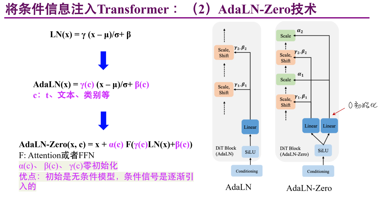
gate 是 SiLU(norm(x)) 产生的门控信号,后面用于 gated residual。具体的AdaRMS类似AdaLN-Zero,把LN换成RMS
② QKV 投影(各自独立,映射到相同的 head_dim)
1
2
3
4
5
6
7
8
9
|
Q_p = q_proj(hidden_p)
K_p = k_proj(hidden_p)
V_p = v_proj(hidden_p)
Q_e = q_proj(hidden_e)
K_e = k_proj(hidden_e)
V_e = v_proj(hidden_e)
|
两个模型各自有独立的 QKV 权重矩阵(PaliGemma 输入 2048 维,Expert 输入 1024 维),但 head_dim 都是 256,所以可以在 head 维度上 concat。
③ 拼接后联合 Attention(关键!)
1
2
3
4
|
Q = cat([Q_p, Q_e], dim=2)
K = cat([K_p, K_e], dim=2)
V = cat([V_p, V_e], dim=2)
|
1
2
3
4
5
6
7
| Q_p: [B, 8, P, 256] Q_e: [B, 8, C, 256]
└── P ──┘ └── C ──┘
\ /
───── cat ─────────
│
Q: [B, 8, P+C, 256]
└─ P+C ─┘
|
然后在这条拼接的序列上做标准的 RoPE + scaled dot-product attention:
1
2
3
4
5
6
7
8
|
Q, K = apply_rotary_pos_emb(Q, K, cos, sin)
scores = Q @ K^T / sqrt(256)
scores = scores + attention_mask_4d
attn = softmax(scores)
output = attn @ V
|
这一行 Q @ K^T 就是 prefix 和 suffix 交叉注意的地方:
Q_p @ K_p^T:prefix 内部注意(双向)Q_p @ K_e^T:被 mask 阻断(prefix 看不见 suffix)Q_e @ K_p^T:suffix 读取 prefix(能看到 vision+text)Q_e @ K_e^T:suffix 内部注意(双向)
④ 拆分回各自的 hidden space + o_proj
1
2
3
4
5
6
7
8
9
|
output: [B, 8, P+C, 256]
out_p = output[:, :, :P, :]
out_e = output[:, :, P:, :]
out_p = o_proj_p(out_p)
out_e = o_proj_e(out_e)
|
⑤ Gated Residual + Post-Attention Norm + MLP(各自独立)
1
2
3
4
5
6
7
8
9
10
11
12
13
14
15
|
out_p = gate_p * hidden_p + (1 - gate_p) * out_p
res_p = out_p.clone()
out_p, gate_p = post_attention_layernorm(out_p, cond=None)
out_p = mlp_p(out_p)
out_p = gate_p * res_p + (1 - gate_p) * out_p
out_e = gate_e * hidden_e + (1 - gate_e) * out_e
res_e = out_e.clone()
out_e, gate_e = post_attention_layernorm(out_e, cond=time_emb)
out_e = mlp_e(out_e)
out_e = gate_e * res_e + (1 - gate_e) * out_e
|
⑥ 回到循环,作为下一层的输入
1
| inputs_embeds = [out_p, out_e]
|
一层完整的数据流图
1
2
3
4
5
6
7
8
9
10
11
12
13
14
15
16
17
18
19
20
21
22
23
24
25
26
27
28
29
30
31
32
33
34
35
36
37
38
| prefix_embs [B,P,Wp] suffix_embs [B,C,We]
│ │
┌──────────┼──────────┐ ┌─────────┼──────────┐
│ input_layernorm │ │ input_layernorm │
│ (adaRMS=None) │ │ (adaRMS=time_emb) │
└─────────────────────┘ └────────────────────┘
│ │
Q_p,K_p,V_p Q_e,K_e,V_e
[B,8,P,256] [B,1,P,256] [B,8,C,256] [B,1,C,256]
│ │
└──────────┬─────────────────┘
│
Q=[B,8,P+C,256]
K=[B,1,P+C,256] ← RoPE 注入
V=[B,1,P+C,256]
│
┌────────▼────────┐
│ Joint Attention │
│ Q@K^T + mask │
│ softmax · V │
└────────┬────────┘
│
[B,8,P+C,256]
,─────────────────.
slice :P slice P:
[B,8,P,256] [B,8,C,256]
│ │
o_proj_p [B,P,Wp] o_proj_e [B,C,We]
│ │
gated_residual gated_residual
│ │
post_attn_layernorm post_attn_layernorm(cond=time_emb)
│ │
mlp_p FFN mlp_e FFN
│ │
gated_residual gated_residual
│ │
prefix_embs [B,P,Wp] suffix_embs [B,C,We]
|
2.3. 推理 Forward Pass
2.3.1. 推理全数据流概览
推理使用 ODE 积分(Euler 方法),从纯噪声逐步去噪:
1
2
3
4
5
6
7
8
9
10
11
12
13
14
15
16
17
18
19
20
21
22
23
24
25
26
27
28
29
30
31
32
33
34
35
36
37
38
39
40
41
42
43
44
45
46
47
48
49
50
51
52
53
54
55
| Inference: sample_actions()
═══════════════════════════════════════════════════════════════════
Step 1: 编码 Prefix(与训练相同)
──────────────────────────────
prefix_embs, prefix_pad_masks, prefix_att_masks = embed_prefix(...)
执行 PaliGemma forward(只做 prefix):
paligemma_with_expert.forward(
inputs_embeds=[prefix_embs, None],
use_cache=True
)
→ prefix_output, past_key_values
⚠️ 关键优化:prefix 只计算一次,KV cache 在后续去噪步骤中复用!
Step 2: 去噪循环 (Euler ODE integration)
─────────────────────────────────────────
dt = -1.0 / num_inference_steps (默认 10 步)
x_t = noise ~ N(0, 1) [B, 50, 32]
for step in range(10):
time = 1.0 + step * dt
┌─ denoise_step(): ────────────────────── ┐
│ ① embed_suffix(x_t, time) │
│ action_in_proj(x_t) → suffix_embs │
│ time → sinusoidal → time_mlp → adamrs│
│ │
│ ② build attention mask │
│ prefix_pad (reuse) + suffix_causal │
│ │
│ ③ Expert Gemma forward │
│ paligemma_with_expert.forward( │
│ inputs_embeds=[None, suffix], │
│ past_key_values=prefix_kv_cache, │ ← 复用 prefix 的 KV!
│ ) │
│ │
│ ④ action_out_proj → v_t │
└─────────────────────────────────────────┘
if RTC enabled:
v_t = rtc_processor.denoise_step(...)
x_t = x_t + dt * v_t
Step 3: 后处理
──────────────
actions = x_t[:, :, :original_action_dim]
Action Queue(n_action_steps=50):
actions [B, 50, act_dim] → 转置 → queue 缓存 50 个 actions
每次 select_action() 从 queue 左侧 pop 一个 [B, act_dim]
|
2.3.2. 去噪 Euler ODE
1
2
3
4
5
6
7
8
9
10
11
12
13
14
15
16
17
18
19
20
21
22
23
24
25
26
27
28
29
30
31
|
Step 2: 去噪循环 (Euler ODE integration)
─────────────────────────────────────────
dt = -1.0 / num_inference_steps (默认 10 步)
x_t = noise ~ N(0, 1) [B, 50, 32]
for step in range(10):
time = 1.0 + step * dt
┌─ denoise_step(): ────────────────────── ┐
│ ① embed_suffix(x_t, time) │
│ action_in_proj(x_t) → suffix_embs │
│ time → sinusoidal → time_mlp → adamrs│
│ │
│ ② build attention mask │
│ prefix_pad (reuse) + suffix_causal │
│ │
│ ③ Expert Gemma forward │
│ paligemma_with_expert.forward( │
│ inputs_embeds=[None, suffix], │
│ past_key_values=prefix_kv_cache, │ ← 复用 prefix 的 KV!
│ ) │
│ │
│ ④ action_out_proj → v_t │
└─────────────────────────────────────────┘
if RTC enabled:
v_t = rtc_processor.denoise_step(...)
x_t = x_t + dt * v_t
|
2.3.3. 动作采样和动作队列
1
2
3
4
5
6
7
| Step 3: 后处理
──────────────
actions = x_t[:, :, :original_action_dim]
Action Queue(n_action_steps=50):
actions [B, 50, act_dim] → 转置 → queue 缓存 50 个 actions
每次 select_action() 从 queue 左侧 pop 一个 [B, act_dim]
|
这是 Action Chunking 的执行逻辑——一次预测多个动作,逐个执行,用完再预测。
1
2
3
4
5
6
|
actions = self.predict_action_chunk(batch)[:, : self.config.n_action_steps]
actions.transpose(0, 1)
|
2.3.3.1. 为什么需要 transpose?
deque.extend(iterable) 沿第一维逐个添加元素:
1
2
3
4
5
|
queue.extend(tensor)
queue.extend(tensor)
|
1
2
3
4
5
6
7
8
9
10
| transpose 前: [B=1, T=10, D=7]
└─────────┬─────────┘
这是一个 tensor
transpose 后: [T=10, B=1, D=7]
├─ [1,7] → deque[0] ← pop 先出
├─ [1,7] → deque[1]
├─ [1,7] → deque[2]
...
└─ [1,7] → deque[9]
|
2.3.3.2. pop 和预测的节奏
1
2
3
4
5
6
7
|
第 1 次 select_action: queue 空 → 预测一次,extend 10 个动作,pop 第 1 个
第 2 次 select_action: queue 还有 9 个 → 直接 pop 第 2 个
...
第 10 次 select_action: queue 还有 1 个 → pop 第 10 个
第 11 次 select_action: queue 空 → 再预测一次,extend 新 10 个,pop 第 1 个
|
1
2
3
4
5
6
7
8
| 时间 ──────────────────────────────────────────────────────────────────────────────────────→
predict (50个) 取前10个执行 predict (50个) 取前10个执行
│ │
▼ ▼
[act₀][act₁][act₂]...[act₉] [act₁₀][act₁₁]...[act₁₉]
↑ pop ↑ pop ↑ pop ↑ pop
t=0 t=9 t=10 t=19
|
一次预测 50 个,使用 10 个再预测。10 步之间不需要重新推理,直接用缓存的 deque。50 个 chunk 比 10 个大的原因是让模型看到更长的时间范围,产生更平滑的轨迹,但不是所有 50 个都执行——它每隔 10 步就重新观察环境、重新规划。
2.4. RTC(Real-Time Chunking)
RTC 解决的是连续 chunk 之间的动作平滑性问题。核心思路:
1
2
3
4
5
6
7
8
| 上一个 chunk 未执行完的部分 (prev_chunk_left_over)
│
▼
对当前去噪步骤施加 guidance:
x1_t = x_t - time * v_t ← 用当前速度预测的下一步
err = (prev_leftover - x1_t) * weights
correction = ∂(err)/∂(x_t) ← 通过 autograd 计算修正方向
v_t = v_t - guidance_weight * correction ← 修正速度场
|
RTCProcessor.get_prefix_weights() 提供多种 attention schedule(ZEROS/ONES/LINEAR/EXP),控制前一个 chunk 对当前 chunk 不同位置的影响力。具体可以参考RTC的论文.
2.5. Post-Processor Pipeline
1
2
3
4
5
6
7
8
9
10
| 模型输出 actions [B, 50, act_dim]
│
▼
[1] UnnormalizerProcessorStep — 逆归一化(QUANTILES unnorm → 原始尺度)
│
▼
[2] DeviceProcessorStep("cpu") — 移回 CPU
│
▼
最终 actions → 发送给 robot.send_action() 或 env.step()
|