Stochastic bandits robust to adversarial corruptions

Meta

Tag: #articles/tags/Computer_Science__Machine_Learning, #articles/tags/Statistics__Machine_Learning, #articles/tags/Computer_Science__Data_Structures_and_Algorithms, #articles/tags/Computer_Science__Computer_Science_and_Game_Theory, #articles/tags/Bandit
citekey: lykourisStochasticBanditsRobust2018
authors: #articles/authors/Thodoris-Lykouris, #articles/authors/Vahab-Mirrokni, #articles/authors/Renato-Paes-Leme
year: 2018/03/25
doi: 10.48550/arXiv.1803.09353
url: http://arxiv.org/abs/1803.09353
conference: #articles/conference/
Journal : #articles/journals/

Abstract

We introduce a new model of stochastic bandits with adversarial corruptions which aims to capture settings where most of the input follows a stochastic pattern but some fraction of it can be adversarially changed to trick the algorithm, e.g., click fraud, fake reviews and email spam. The goal of this model is to encourage the design of bandit algorithms that (i) work well in mixed adversarial and stochastic models, and (ii) whose performance deteriorates gracefully as we move from fully stochastic to fully adversarial models. In our model, the rewards for all arms are initially drawn from a distribution and are then altered by an adaptive adversary. We provide a simple algorithm whose performance gracefully degrades with the total corruption the adversary injected in the data, measured by the sum across rounds of the biggest alteration the adversary made in the data in that round; this total corruption is denoted by $C$. Our algorithm provides a guarantee that retains the optimal guarantee (up to a logarithmic term) if the input is stochastic and whose performance degrades linearly to the amount of corruption $C$, while crucially being agnostic to it. We also provide a lower bound showing that this linear degradation is necessary if the algorithm achieves optimal performance in the stochastic setting (the lower bound works even for a known amount of corruption, a special case in which our algorithm achieves optimal performance without the extra logarithm).

笔记与思考

Setting

protocol

More formally, the protocol between learner and adversary, at each round $t = 1 \dots T$, is as follows:

1. The learner picks a distribution $w^t$ over the $K$ arms.
2. Stochastic rewards are drawn for each arm: $r^t_S(a) \sim \mathcal{F}(a)$.
3. The adversary observes the realizations of $r^t_S(a)$ as well as rewards and choices of the learner in previous steps and returns a corrupted reward $r^t(a) \in [0, 1]$.
4. The learner draws arm $a^t \sim w^t$ and observes $r^t(a^t)$.

• We refer to $\max_a |r^t(a) - r^t_S(a)|$ as the amount of corruption injected in round $t$. The instance is $C$-corrupted if the total injected corruption is at most $C$ for all realizations of the random variables:

$\sum_t \max_a |r^t(a) - r^t_S(a)| \leq C$

• Note that the adversary is assumed to be adaptive

  • In adaptive setting, the corruptions are not necessarily i.i.d. across rounds but only conditional independence (conditioned on the history). That’s why we introduce the concentration inequality in the pf of Lemma 3.3.

• The Difference corrupted stochastic bandit and slow varing bandit

Corrupted

the adversary corruption is more like a noise and it won’t bias the true reward mean.
focus on how to sample

Slow vary

the variation budget constrains the cumulative shift in the true reward means.
focus on how to forget

---

Regret

$Reg = \underset{a}{\max}\sum_t r^t(a)-r^t(a_t)$, noted that $r^t(a)=r_{\mathcal{S}}^t(a)+r^t_{\mathcal{C}}(a)$

high Probablity bound

1. $\mathbb{P}[Reg < R(T, δ)] > 1 − δ$, which you should consider the variance of the reward (the true reward may higher than empirical reward for suboptimal arms, and … for optimal arm)
2. the arm who has the best cumulative reward shouldn’t be assumed to have the optimal mean, as we consider the realized cumulative reward instead of the empirical one.

pseudo bound

1. $PseudoReg=\underset{a}{\max}\mathbb{E}(\sum_t r^t(a)-r^t(a_t))$
2. the stochastic pseudo bound can be calculated by $\Delta(a)N(a)$
3. it’s weaker than the high prob. bound.

connection

1. Fortunately, the difference(variance) between realization and the expectation is at most $\sqrt{N(a)\log\left( \frac{2kT}{\delta} \right)}$ which can be derived by the hoeffding bound.
2. What’s more, the variance can be bounded by $N(a)\Delta(a)$
3. However, by the same argument as above arm $a^⋆$ is with high probability at most $N(a^′) · ∆(a^′)$ below its expectation and the ex post optimal arm is at most this much above its expectation. This gives a bound of $N(a^′)∆(a^′)$ that is caused by the case where $a^⋆$ is not the ex post optimal arm.

Algorithm

proof lines

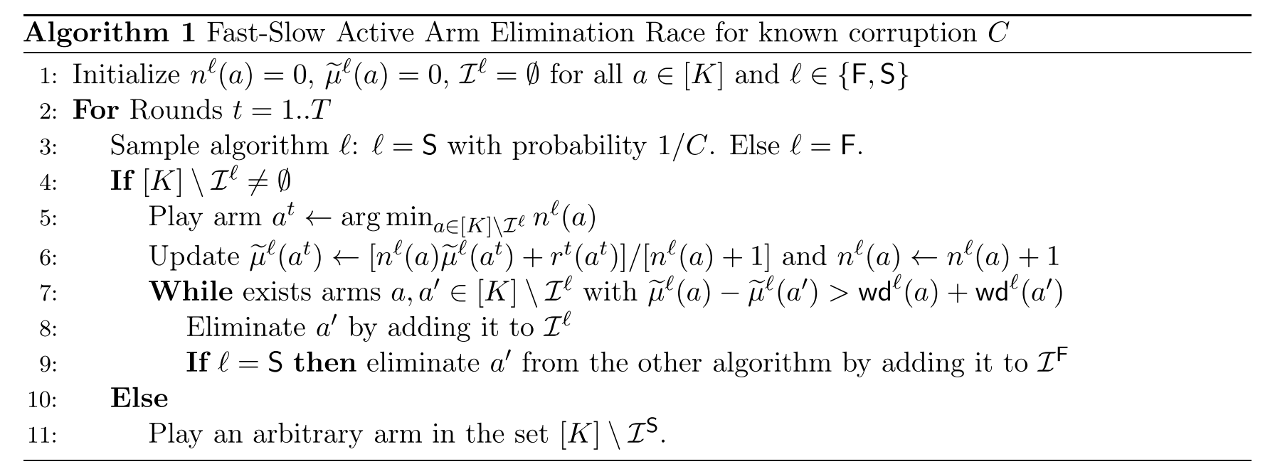
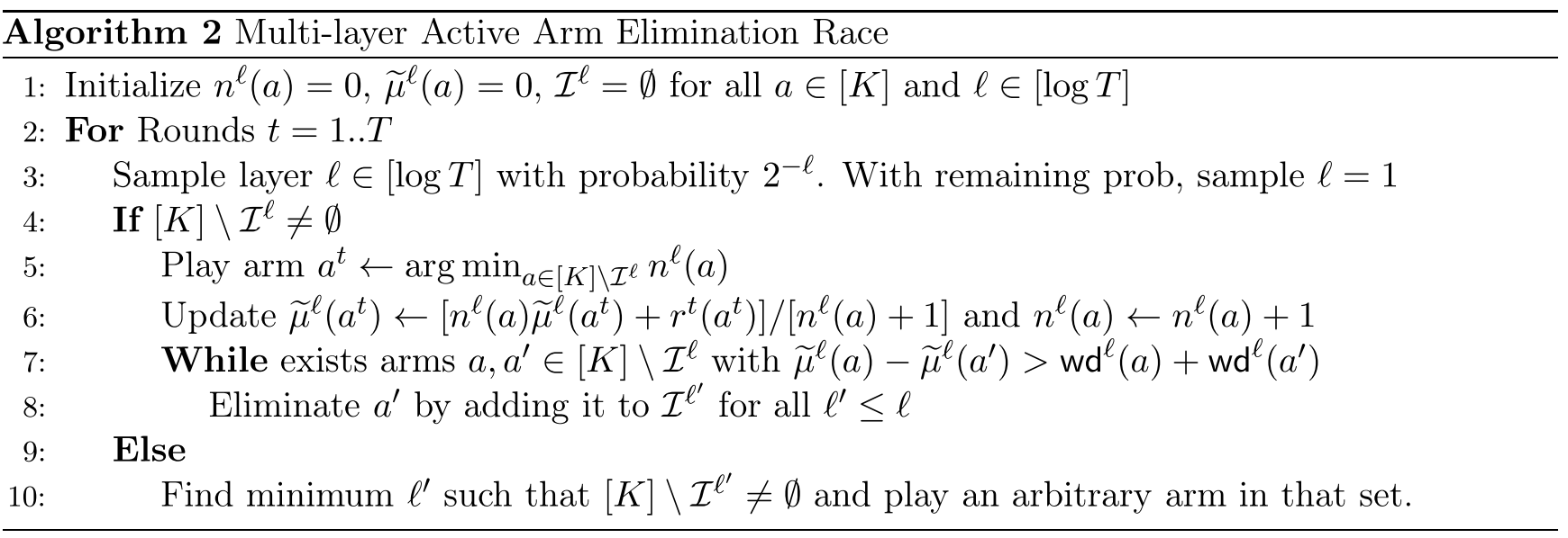
• Fast layers can detect quickly in low corruption settings and Slow layers eliminate arms carefully with higher accuracy and correct or confirm the fast layers’ decisions.
• subsampling(Lemma3.3) : Slow layers is raised with probability of $\frac{1}{c}$, so that the slow layer suffer $O(1)$ corruption in expectation and corruption level can be bound by $2\sqrt{\log\left( \frac{KT}{\delta} \right)}$ at high probability. So it’s easy to estimate C.

Result

• key point is that we can calculate the $N_{S}(a)$ in appropriate Slow layer ($2^{-\mathcal{l}}\approx\frac{1}{C}$), and then we can calculate the Fast layers’ $N_{F}(a)$ by $N_{S}(a)$.
  • more specifically, the last time Fast layers pull arm $a$, is at most $C\cdot K\cdot N_{S}(a)$ in expectation.
    • $K\cdot N_{S}(a)$ denote the terminal time step of pulling arm $a$ in the slow time scale.
    • With probabilty at most $\frac{1}{c}$ of sampling the appropriate Slow layer, we should multiply by $C$ to convert the result to the Fast tiem scale.
  • we should quantify the number of fast-layer moves $M$ required to trigger a slow layer with high probability.

ELIM with enlarged interval
Fast & Slow layer instance
Multi-layer instance (agnostic)

takeaway

1. subsampling : preventing algorithm suffer too many corruptions and effeciently estimate corruption level
2. multi-scale : maintain both stochastic and corrupted ability