Meta
Tag : #articles/tags/Computer_Science__Machine_Learning, #articles/tags/Statistics__Machine_Learning, #articles/tags//unreadcitekey : fanDecentralizedAsynchronousMultiplayer2025authors : #articles/authors/Jingqi-Fan, #articles/authors/Canzhe-Zhao, #articles/authors/Shuai-Li, #articles/authors/Siwei-Wangyear : 2025/09/30doi : 10.48550/arXiv.2509.25824url : http://arxiv.org/abs/2509.25824 conference : #articles/conference/Journal : #articles/journals/
Abstract
In recent years, multi-player multi-armed bandits (MP-MAB) have been extensively studied due to their wide applications in cognitive radio networks and Internet of Things systems. While most existing research on MP-MAB focuses on synchronized settings, real-world systems are often decentralized and asynchronous, where players may enter or leave the system at arbitrary times, and do not have a global clock. This decentralized asynchronous setting introduces two major challenges. First, without a global time, players cannot implicitly coordinate their actions through time, making it difficult to avoid collisions. Second, it is important to detect how many players are in the system, but doing so may cost a lot. In this paper, we address the challenges posed by such a fully asynchronous setting in a decentralized environment. We develop a novel algorithm in which players adaptively change between exploration and exploitation. During exploration, players uniformly pull their arms, reducing the probability of collisions and effectively mitigating the first challenge. Meanwhile, players continue pulling arms currently exploited by others with a small probability, enabling them to detect when a player has left, thereby addressing the second challenge. We prove that our algorithm achieves a regret of O ( T log T + log T / Δ 2 ) \mathcal{O}(\sqrt{T \log T} + {\log T}/{Δ^2}) O ( T log T + log T / Δ 2 ) Δ Δ Δ
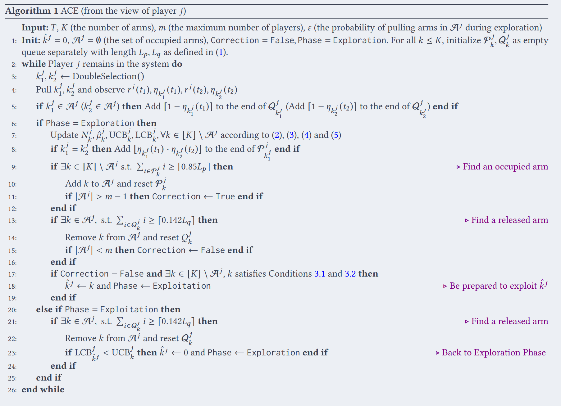
k ^ j \hat k^j k ^ j A j \mathcal{A}^j A j ∣ A j ∣ > m − 1 |\mathcal{A}^j|>m-1 ∣ A j ∣ > m − 1 occupy: 代表的是以高概率利用这arm
release: 代表之前利用某个arm,此时要停止利用,要么离开系统
P k j \mathcal{P}^j_k P k j k 1 j = k 2 j k^j_1=k^j_2 k 1 j = k 2 j η k 1 j ( t 1 ) ⋅ η k 2 j ( t 2 ) \eta_{k^j_1}(t_1)\cdot\eta_{k^j_2}(t_2) η k 1 j ( t 1 ) ⋅ η k 2 j ( t 2 ) A j \mathcal{A}^j A j
∣ P k j ∣ : = L p = ⌈ 866 l n ( T ) ⌉ |\mathcal{P}^j_k | := Lp = ⌈866 ln(T )⌉ ∣ P k j ∣ : = L p = ⌈ 8 6 6 l n ( T ) ⌉ ∑ i ∈ P k j i ≥ ⌈ 0.85 L p ⌉ \sum _{i∈P^j_k} i≥ ⌈0.85Lp ⌉ ∑ i ∈ P k j i ≥ ⌈ 0 . 8 5 L p ⌉
Q k j \mathcal{Q}^j_k Q k j k 2 j k^j_2 k 2 j A j \mathcal{A}^j A j A j \mathcal{A}^j A j
∣ Q k j ∣ : = L q = ⌈ 570 l n ( T ) ⌉ |\mathcal{Q} ^j_ k | := Lq = ⌈570 ln(T )⌉ ∣ Q k j ∣ : = L q = ⌈ 5 7 0 l n ( T ) ⌉ ∑ i ∈ Q k j i ≥ ⌈ 0.142 L q ⌉ \sum_{i∈Q^j _k} i ≥ ⌈0.142Lq⌉ ∑ i ∈ Q k j i ≥ ⌈ 0 . 1 4 2 L q ⌉
注意,
P \mathcal{P} P 和
Q \mathcal{Q} Q 都是队列, 也就是他实际上是一个先进先出的结构!
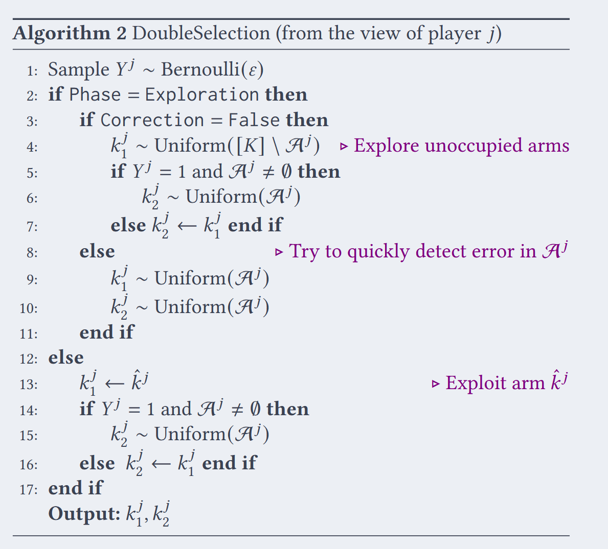
对于任意一个在exploration phase 的agent j j j k k k 1 m \frac{1}{m} m 1
P \mathcal{P} P Q \mathcal{Q} Q 我们必须从两个event开始
E 1 : = { ∃ t ∈ T j , j ≤ M , k ≤ K : ∣ ∑ τ p = τ L p + τ C k j ( t k , p j ( τ p ) ) − ∑ τ p = τ L p + τ E [ C k j ( t k , p j ( τ p ) ) ∣ F τ p − 1 ] ∣ ≥ 0.034 L p } , E 2 : = { ∃ t ∈ T j , j ≤ M , k ≤ K : ∣ ∑ τ q = τ L q + τ D k j ( t k , q j ( τ q ) ) − ∑ τ q = τ L q + τ E [ D k j ( t k , q j ( τ q ) ) ∣ F τ q − 1 ] ∣ ≥ 0.0419 L q } \begin{aligned}
\mathcal{E}_1 &:= \left\{ \exists t \in \mathcal{T}^j, j \le M, k \le K : \left| \sum_{\tau_p = \tau}^{L_p + \tau} C_k^j (t_{k,p}^j(\tau_p)) - \sum_{\tau_p = \tau}^{L_p + \tau} \mathbb{E} [C_k^j (t_{k,p}^j(\tau_p)) | \mathcal{F}_{\tau_{p-1}}] \right| \ge 0.034 L_p \right\}, \\
\mathcal{E}_2 &:= \left\{ \exists t \in \mathcal{T}^j, j \le M, k \le K : \left| \sum_{\tau_q = \tau}^{L_q + \tau} D_k^j (t_{k,q}^j(\tau_q)) - \sum_{\tau_q = \tau}^{L_q + \tau} \mathbb{E} [D_k^j (t_{k,q}^j(\tau_q)) | \mathcal{F}_{\tau_{q-1}}] \right| \ge 0.0419 L_q \right\}
\end{aligned} E 1 E 2 : = ⎩ ⎨ ⎧ ∃ t ∈ T j , j ≤ M , k ≤ K : ∣ ∣ ∣ ∣ ∣ ∣ τ p = τ ∑ L p + τ C k j ( t k , p j ( τ p ) ) − τ p = τ ∑ L p + τ E [ C k j ( t k , p j ( τ p ) ) ∣ F τ p − 1 ] ∣ ∣ ∣ ∣ ∣ ∣ ≥ 0 . 0 3 4 L p ⎭ ⎬ ⎫ , : = ⎩ ⎨ ⎧ ∃ t ∈ T j , j ≤ M , k ≤ K : ∣ ∣ ∣ ∣ ∣ ∣ τ q = τ ∑ L q + τ D k j ( t k , q j ( τ q ) ) − τ q = τ ∑ L q + τ E [ D k j ( t k , q j ( τ q ) ) ∣ F τ q − 1 ] ∣ ∣ ∣ ∣ ∣ ∣ ≥ 0 . 0 4 1 9 L q ⎭ ⎬ ⎫
C k j ( ⋅ ) C^j_k(\cdot) C k j ( ⋅ ) τ p \tau_p τ p t k j ( ⋅ ) t^j_k(\cdot) t k j ( ⋅ ) 整个event代表的是实际上的队列长度和期望中的队列长度的差, 很大.
为了使得这两个event的发生概率很小, 通过集中不等式 , 可以得到相应的长度L p L_p L p LemmaB.3 )
对于P \mathcal{P} P 对于thredhold的考量是为了区分真的有agent occupy arm k, 和没有agent occupy arm k.
对于有agent occupy arm k 的情况由于exploit的时候至少会有ϵ \epsilon ϵ 1 − ϵ 1-\epsilon 1 − ϵ ∑ τ p = τ L p + τ E [ C k j ( t k , p j ( τ p ) ) ∣ F τ p − 1 ] ≥ 0.9 L p . \sum_{\tau_p=\tau}^{L_p+\tau} \mathbb{E} \left[ C_k^j (t_{k,p}^j(\tau_p)) \mid \mathcal{F}_{\tau_{p-1}} \right] \ge 0.9 L_p . ∑ τ p = τ L p + τ E [ C k j ( t k , p j ( τ p ) ) ∣ F τ p − 1 ] ≥ 0 . 9 L p .
而对于没有agent occupy arm k 的情况下, 由于任意一个arm k被pull的概率不超过1 m \frac{1}{m} m 1 1 − ∏ j ′ ≠ j : j ′ is active ( 1 − 1 m ) ≤ 1 − ( 1 − 1 m ) m ≤ 1 − 1 2 e ≤ 0.816. 1 - \prod_{j' \neq j: j' \text{ is active}} \left(1 - \frac{1}{m}\right) \le 1 - \left(1 - \frac{1}{m}\right)^m \le 1 - \frac{1}{2e} \le 0.816 . 1 − ∏ j ′ = j : j ′ is active ( 1 − m 1 ) ≤ 1 − ( 1 − m 1 ) m ≤ 1 − 2 e 1 ≤ 0 . 8 1 6 . ∑ τ p = τ L p + τ E [ C k j ( t k , p j ( τ p ) ) ∣ F τ p − 1 ] ≤ 0.816 L p . \sum_{\tau_p=\tau}^{L_p+\tau} \mathbb{E} \left[ C_k^j \left(t_{k,p}^j(\tau_p)\right) \mid \mathcal{F}_{\tau_{p-1}} \right] \le 0.816L_p . ∑ τ p = τ L p + τ E [ C k j ( t k , p j ( τ p ) ) ∣ F τ p − 1 ] ≤ 0 . 8 1 6 L p .
根据上面两个序列长度的分析, 接着我们考虑到方差的影响, 我们直接取中点作为thredhold, 这样的话两边方差的radius就一样了, 中点也就是0.85 L p 0.85L_p 0 . 8 5 L p
相似的分析对Q \mathcal{Q} Q
除此之外, 我们还可以通过这些分析出最大需要多少步才能把arm正确加入A j A^j A j A j A^j A j O ( log T ) \mathcal{O}(\log T) O ( log T )
要转移到exploitation需要满足两个condition:
Condition 3.1: 由于在exploit阶段并不是每个时间都pull k ^ j \hat k^j k ^ j k ^ j \hat k^j k ^ j 如果两步都不碰, 那说明确实没有人occupy
Condition 3.2: 经典的explore-then-commit式算法的exploit的条件
condition 3.2 实际上是一个标准的explore-then-commit算法的条件, 这个条件通常可以直接转换为$$\mu_k-\mu_{k’}\geq4\times \max_{k,k’} \textbf{Confidence interval radius}$$通过这个条件可以计算出至少需要多少个sample才能把一些arm给eliminate.
在满足了3.2. 之后需要满足3.1. 还需要采样的步数, 可以把这个建模成每一步选中arm k的概率为p, 而其他agent不选择arm k, 随机变量为这个时间发生第一次的轮数N, 求N的期望E [ T c ] \mathbb{E}[T_{c}] E [ T c ] Lemma4.2 )
G 1 j : = { t ∈ T j : ∃ j ′ ≠ j , j ′ ∈ [ M ] , ∃ k ≤ K , k ∉ A j ( t ) , k ^ j ′ = k } , G 2 j : = { t ∈ T j : ∃ k ∈ A j ( t ) , ∀ j ′ ≠ j , j ′ ∈ [ M ] , k ^ j ′ ≠ k } , \begin{aligned}
\mathcal{G}_1^j &:= \left\{ t \in \mathcal{T}^j : \exists j' \neq j, j' \in [M], \exists k \le K, k \notin \mathcal{A}^j(t), \hat{k}^{j'} = k \right\} , \\
\mathcal{G}_2^j &:= \left\{ t \in \mathcal{T}^j : \exists k \in \mathcal{A}^j(t), \forall j' \neq j, j' \in [M], \hat{k}^{j'} \neq k \right\} ,
\end{aligned} G 1 j G 2 j : = { t ∈ T j : ∃ j ′ = j , j ′ ∈ [ M ] , ∃ k ≤ K , k ∈ / A j ( t ) , k ^ j ′ = k } , : = { t ∈ T j : ∃ k ∈ A j ( t ) , ∀ j ′ = j , j ′ ∈ [ M ] , k ^ j ′ = k } ,
这两个事件分别代表着对于被exploit的arm没有被检测到A j \mathcal{A^j} A j A j \mathcal{A^j} A j
≤ ∑ j ≤ M ∑ t = T start j T end j E [ 1 − 1 [ π j ( t ) ≤ m t , η j ( t ) = 0 ] ∣ E 0 ‾ ] + ∑ j ≤ M T j Pr [ E 0 ] ( 12 ) ≤ ∑ j ≤ M E [ ∣ G 2 j ∣ ∣ E 0 ‾ ] ⏟ A + ∑ j ≤ M ∑ t ∈ T exp j E [ 1 [ t ∉ G 1 j ∪ G 2 j ] ∣ E 0 ‾ ] ⏟ B + ∑ j ≤ M ∑ t ∈ T exp j E [ 1 [ t ∈ G 1 j ] ∣ E 0 ‾ ] ⏟ C + ∑ j ≤ M T j Pr [ E 0 ] ⏟ E + ∑ j ≤ M ∑ t ∈ T explt j E [ ( 1 − 1 [ π j ( t ) ≤ m t , η π j ( t ) ( t ) = 0 ] ) 1 [ t ∉ G 2 j ] ∣ E 0 ‾ ] ⏟ D . \begin{aligned}
&\le \sum_{j \le M} \sum_{t=T_{\text{start}}^j}^{T_{\text{end}}^j} \mathbb{E} \left[ 1 - \mathbb{1}[\pi^j(t) \le m_t, \eta^j(t) = 0] \mid \overline{\mathcal{E}_0} \right] + \sum_{j \le M} T^j \Pr[\mathcal{E}_0] \quad (12) \\
&\le \underbrace{\sum_{j \le M} \mathbb{E} \left[ |\mathcal{G}_2^j| \mid \overline{\mathcal{E}_0} \right]}_{A} + \underbrace{\sum_{j \le M} \sum_{t \in \mathcal{T}_{\text{exp}}^j} \mathbb{E} \left[ \mathbb{1}[t \notin \mathcal{G}_1^j \cup \mathcal{G}_2^j] \mid \overline{\mathcal{E}_0} \right]}_{B} \\
&+ \underbrace{\sum_{j \le M} \sum_{t \in \mathcal{T}_{\text{exp}}^j} \mathbb{E} \left[ \mathbb{1}[t \in \mathcal{G}_1^j] \mid \overline{\mathcal{E}_0} \right]}_{C} + \underbrace{\sum_{j \le M} T^j \Pr[\mathcal{E}_0]}_{E} \\
&+ \underbrace{\sum_{j \le M} \sum_{t \in \mathcal{T}_{\text{explt}}^j} \mathbb{E} \left[ \left( 1 - \mathbb{1}[\pi^j(t) \le m_t, \eta_{\pi^j(t)}(t) = 0] \right) \mathbb{1}[t \notin \mathcal{G}_2^j] \mid \overline{\mathcal{E}_0} \right]}_{D} .
\end{aligned} ≤ j ≤ M ∑ t = T start j ∑ T end j E [ 1 − 1 [ π j ( t ) ≤ m t , η j ( t ) = 0 ] ∣ E 0 ] + j ≤ M ∑ T j Pr [ E 0 ] ( 1 2 ) ≤ A j ≤ M ∑ E [ ∣ G 2 j ∣ ∣ E 0 ] + B j ≤ M ∑ t ∈ T exp j ∑ E [ 1 [ t ∈ / G 1 j ∪ G 2 j ] ∣ E 0 ] + C j ≤ M ∑ t ∈ T exp j ∑ E [ 1 [ t ∈ G 1 j ] ∣ E 0 ] + E j ≤ M ∑ T j Pr [ E 0 ] + D j ≤ M ∑ t ∈ T explt j ∑ E [ ( 1 − 1 [ π j ( t ) ≤ m t , η π j ( t ) ( t ) = 0 ] ) 1 [ t ∈ / G 2 j ] ∣ E 0 ] .
(12)式分解, 实际上是:
condition on E ˉ 0 \bar{\mathcal{E}}_{0} E ˉ 0 ∈ [ m t ] \in[m_t] ∈ [ m t ]
由于E ˉ 0 \bar{\mathcal{E}}_{0} E ˉ 0
A: 所有agent因无人利用arm残留在A j \mathcal{A}^j A j
B: 在explore phase, exploit的arm被检测到A j \mathcal{A^j} A j A j \mathcal{A^j} A j
C: 在explore phase, exploit的arm被没有检测到A j \mathcal{A^j} A j
D: 在exploit phase, 选择了最优arm ∈ [ m t ] \in[m_t] ∈ [ m t ] A j \mathcal{A^j} A j
对于B还可以进一步分解:
≤ ∑ j ≤ M ∑ t ∈ T exp j E [ ∑ k ∉ A j ( t ) 1 [ π j ( t ) = k ] 1 [ t ∉ G 1 j ∪ G 2 j ] 1 { π j ( t ) ∈ K 2 ( t ) } | E 0 ‾ ∩ E 3 ‾ ] ⏟ B 1 + ∑ j ≤ M ∑ t ∈ T exp j E [ ∑ k ∈ A j ( t ) 1 [ π j ( t ) = k ] 1 [ t ∉ G 1 j ∪ G 2 j ] 1 { π j ( t ) ∈ K 2 ( t ) } | E 0 ‾ ∩ E 3 ‾ ] ⏟ B 2 + ∑ j ≤ M ∑ t ∈ T exp j E [ ∑ k ≤ K 1 [ π j ( t ) = k ] 1 [ t ∉ G 1 j ∪ G 2 j ] 1 { π j ( t ) ∉ K 2 ( t ) , π j ( t ) ∈ K 1 ( t ) } | E 0 ‾ ∩ E 3 ‾ ] ⏟ B 3 + ∑ j ≤ M ∑ t ∈ T exp j E [ ∑ k ≤ K 1 [ π j ( t ) = k ] 1 [ t ∉ G 1 j ∪ G 2 j ] 1 { π j ( t ) ∉ K 2 ( t ) , π j ( t ) ∉ K 1 ( t ) } | E 0 ‾ ∩ E 3 ‾ ] ⏟ B 4 + ∑ j ≤ M T exp j Pr [ E 3 ] ⏟ B 5 . \begin{aligned}
\le &\underbrace{\sum_{j \le M} \sum_{t \in \mathcal{T}_{\text{exp}}^j} \mathbb{E} \left[ \sum_{k \notin \mathcal{A}^j(t)} \mathbb{1}[\pi^j(t) = k] \mathbb{1}[t \notin \mathcal{G}_1^j \cup \mathcal{G}_2^j] \mathbb{1}\{\pi^j(t) \in \mathcal{K}_2(t)\} \middle| \overline{\mathcal{E}_0} \cap \overline{\mathcal{E}_3} \right]}_{B_1} \\
&+ \underbrace{\sum_{j \le M} \sum_{t \in \mathcal{T}_{\text{exp}}^j} \mathbb{E} \left[ \sum_{k \in \mathcal{A}^j(t)} \mathbb{1}[\pi^j(t) = k] \mathbb{1}[t \notin \mathcal{G}_1^j \cup \mathcal{G}_2^j] \mathbb{1}\{\pi^j(t) \in \mathcal{K}_2(t)\} \middle| \overline{\mathcal{E}_0} \cap \overline{\mathcal{E}_3} \right]}_{B_2} \\
&+ \underbrace{\sum_{j \le M} \sum_{t \in \mathcal{T}_{\text{exp}}^j} \mathbb{E} \left[ \sum_{k \le K} \mathbb{1}[\pi^j(t) = k] \mathbb{1}[t \notin \mathcal{G}_1^j \cup \mathcal{G}_2^j] \mathbb{1}\{\pi^j(t) \notin \mathcal{K}_2(t), \pi^j(t) \in \mathcal{K}_1(t)\} \middle| \overline{\mathcal{E}_0} \cap \overline{\mathcal{E}_3} \right]}_{B_3} \\
&+ \underbrace{\sum_{j \le M} \sum_{t \in \mathcal{T}_{\text{exp}}^j} \mathbb{E} \left[ \sum_{k \le K} \mathbb{1}[\pi^j(t) = k] \mathbb{1}[t \notin \mathcal{G}_1^j \cup \mathcal{G}_2^j] \mathbb{1}\{\pi^j(t) \notin \mathcal{K}_2(t), \pi^j(t) \notin \mathcal{K}_1(t)\} \middle| \overline{\mathcal{E}_0} \cap \overline{\mathcal{E}_3} \right]}_{B_4} \\
&+ \underbrace{\sum_{j \le M} T_{\text{exp}}^j \Pr[\mathcal{E}_3]}_{B_5} .
\end{aligned} ≤ B 1 j ≤ M ∑ t ∈ T exp j ∑ E ⎣ ⎡ k ∈ / A j ( t ) ∑ 1 [ π j ( t ) = k ] 1 [ t ∈ / G 1 j ∪ G 2 j ] 1 { π j ( t ) ∈ K 2 ( t ) } ∣ ∣ ∣ ∣ ∣ ∣ E 0 ∩ E 3 ⎦ ⎤ + B 2 j ≤ M ∑ t ∈ T exp j ∑ E ⎣ ⎡ k ∈ A j ( t ) ∑ 1 [ π j ( t ) = k ] 1 [ t ∈ / G 1 j ∪ G 2 j ] 1 { π j ( t ) ∈ K 2 ( t ) } ∣ ∣ ∣ ∣ ∣ ∣ E 0 ∩ E 3 ⎦ ⎤ + B 3 j ≤ M ∑ t ∈ T exp j ∑ E [ k ≤ K ∑ 1 [ π j ( t ) = k ] 1 [ t ∈ / G 1 j ∪ G 2 j ] 1 { π j ( t ) ∈ / K 2 ( t ) , π j ( t ) ∈ K 1 ( t ) } ∣ ∣ ∣ ∣ ∣ E 0 ∩ E 3 ] + B 4 j ≤ M ∑ t ∈ T exp j ∑ E [ k ≤ K ∑ 1 [ π j ( t ) = k ] 1 [ t ∈ / G 1 j ∪ G 2 j ] 1 { π j ( t ) ∈ / K 2 ( t ) , π j ( t ) ∈ / K 1 ( t ) } ∣ ∣ ∣ ∣ ∣ E 0 ∩ E 3 ] + B 5 j ≤ M ∑ T exp j Pr [ E 3 ] .
使用是否满足condition3.1(不满足3.1, K 1 \mathcal{K}_{1} K 1 K 2 \mathcal{K}_{2} K 2
B1 : 可以直接从(LemmaB.8 )得到相关结论, 这里还要考虑A j \mathcal{A}^j A j
B2: ∑ j ≤ M ε T e x p j \sum_{j≤M} εT ^j_{ exp} ∑ j ≤ M ε T e x p j
B3: 可以从E [ T c ] \mathbb{E}[ T_c] E [ T c ]
这两个term实际上都是由于检测延误所造成的regret, 实际上在上面的P \mathcal{P} P Q \mathcal{Q} Q
≤ ∑ j ≤ M ∑ t ∈ T explt j E [ η k ^ j ( t ) 1 [ π j ( t ) = k ^ j , ∃ j ′ ≠ j , j ′ ∈ [ M ] , k ^ j ∉ A j ′ ( t ) , t ∉ G 2 j ] ∣ E 0 ‾ ] ⏟ D 1 + ∑ j ≤ M ∑ t ∈ T explt j E [ η k ^ j ( t ) 1 [ π j ( t ) = k ^ j , ∀ j ′ ≠ j , j ′ ∈ [ M ] , k ^ j ∈ A j ′ ( t ) , t ∉ G 2 j ] ∣ E 0 ‾ ] ⏟ D 2 + ∑ j ≤ M ε T explt j , \begin{aligned} \le &\underbrace{\sum_{j \le M} \sum_{t \in \mathcal{T}_{\text{explt}}^j} \mathbb{E} \left[ \eta_{\hat{k}^j}(t) \mathbb{1} [\pi^j(t) = \hat{k}^j, \exists j' \neq j, j' \in [M], \hat{k}^j \notin \mathcal{A}^{j'}(t), t \notin \mathcal{G}_2^j] \mid \overline{\mathcal{E}_0} \right]}_{D_1} \\ &+ \underbrace{\sum_{j \le M} \sum_{t \in \mathcal{T}_{\text{explt}}^j} \mathbb{E} \left[ \eta_{\hat{k}^j}(t) \mathbb{1} [\pi^j(t) = \hat{k}^j, \forall j' \neq j, j' \in [M], \hat{k}^j \in \mathcal{A}^{j'}(t), t \notin \mathcal{G}_2^j] \mid \overline{\mathcal{E}_0} \right]}_{D_2} \\ &+ \sum_{j \le M} \varepsilon T_{\text{explt}}^j , \end{aligned}
≤ D 1 j ≤ M ∑ t ∈ T explt j ∑ E [ η k ^ j ( t ) 1 [ π j ( t ) = k ^ j , ∃ j ′ = j , j ′ ∈ [ M ] , k ^ j ∈ / A j ′ ( t ) , t ∈ / G 2 j ] ∣ E 0 ] + D 2 j ≤ M ∑ t ∈ T explt j ∑ E [ η k ^ j ( t ) 1 [ π j ( t ) = k ^ j , ∀ j ′ = j , j ′ ∈ [ M ] , k ^ j ∈ A j ′ ( t ) , t ∈ / G 2 j ] ∣ E 0 ] + j ≤ M ∑ ε T explt j ,
其中D 1 D_{1} D 1 C C C A j \mathcal{A^j} A j
而D 2 D_{2} D 2 ϵ \epsilon ϵ
连续pull两个arm, k 1 j k^j_1 k 1 j k 2 j k^j_2 k 2 j k 2 j k^j_2 k 2 j A j \mathcal{A}^j A j
同时在探索的时候也是, 存在一定的概率使得k 2 j k_2^j k 2 j A j \mathcal{A}^j A j
为什么两个Queue的长度分别设定为这样?
为什么UCB和LCB的系数里有3 \sqrt{3} 3
对于LemmaB.6中情况2, 如果说比L p L_p L p
因为整个队列的长度就是L p L_p L p
设置的队列触发阈值不是越小越好吗?为什么要设置在中点附近?
在这里, 使用的uniform是round robin还是随机的采样? 如果是round robin会不会导致很多arm在exploration的时候同步而导致的持续collision的问题?
takeaway
几何分布: 一件事发生的概率为p, 他在第n次才首次发生的期望 E ( n ) = 1 p \mathbb{E}(n)=\frac{1}{p} E ( n ) = p 1
全期望公式: E [ X ( t ) ] = E [ X ( t ) ∣ E 0 ‾ ] Pr [ E 0 ‾ ] + E [ X ( t ) ∣ E 0 ] Pr [ E 0 ] \mathbb{E}[X(t)] = \mathbb{E}[X(t) \mid \overline{\mathcal{E}_0}] \Pr[\overline{\mathcal{E}_0}] + \mathbb{E}[X(t) \mid \mathcal{E}_0] \Pr[\mathcal{E}_0] E [ X ( t ) ] = E [ X ( t ) ∣ E 0 ] Pr [ E 0 ] + E [ X ( t ) ∣ E 0 ] Pr [ E 0 ]