What Makes a Good Prune Maximal Unstructured Pruning for Maximal Cosine Similarity
Meta
Tag: #articles/tags//unread
citekey: mason-williamsWhatMakesGood2023
authors: #articles/authors/Gabryel-Mason-Williams, #articles/authors/Fredrik-Dahlqvist
year: 2023/10/13
doi:
url: https://openreview.net/forum?id=jsvvPVVzwf
conference: #articles/conference/The_Twelfth_International_Conference_on_Learning_Representations
Journal : #articles/journals/
Abstract
Pruning is an effective method to reduce the size of deep neural network models, maintain accuracy, and, in some cases, improve the network’s overall performance. However, the mechanisms underpinning pruning remain unclear. Why can different methods prune by different percentages yet achieve similar performance? Why can we not prune at the start of training? Why are some models more amenable to being pruned than others? Given a model, what is the maximum amount it can be pruned before significantly affecting the performance? This paper explores and answers these questions from the global unstructured magnitude pruning perspective with one epoch of fine-tuning. We develop the idea that cosine similarity is an effective proxy measure for functional similarity between the parent and the pruned network. We prove that the L1 pruning method is optimal when pruning by cosine similarity. We show that the higher the kurtosis of a model’s parameter distribution, the more it can be pruned while maintaining performance. Finally, we present a simple method to determine the optimal amount by which a network can be L1-pruned based on its parameter distribution. The code demonstrating the method is available at https://github.com/gmw99/what_makes_a_good_prune
Note
- Cosine similarity allows us to compare pruning methods as it is a good proxy measure for functional similarity.
- The L1 magnitude pruning method is optimal for maintaining maximal cosine similarity.
- Maintaining a high cosine similarity with the parent network ensures improved accuracy or limited drop-off in performance.
- Neural networks are brittle, i.e. highly sensitive to changes in high-magnitude parameters.
- The higher the kurtosis of a model’s parameter distribution, the more it can be pruned while maintaining performance.
1. method
- 其中 和 分别是把一个权重 be flattened by concatenation to form a vector representation of the neural network parameters, 对于全局剪枝需要把每一层的全部拼起来, 实际上等价于 也就是最小化
2. experiment
2.1. USING COSINE SIMILARITY TO COMPARE PRUNING METHODS AND OPTIMAL PRUNING
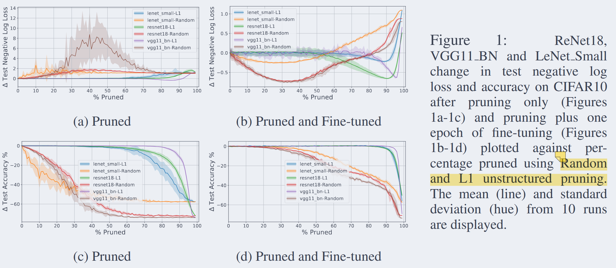
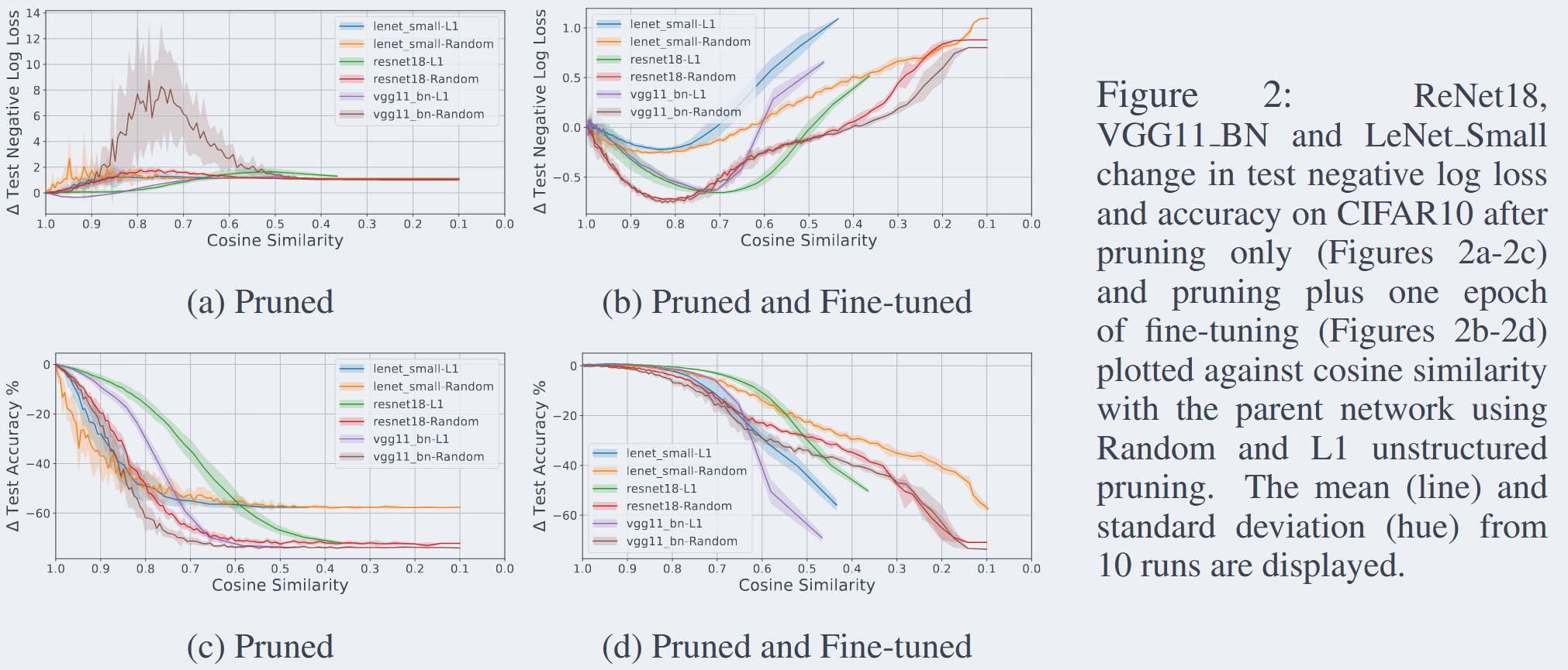
- 从这个两个实验可以看出来保持余弦相似度可以使得模型性能大幅下降的临界剪枝率延后
- 在固定余弦相似性的情况下, 模型的性能几乎和剪枝的方法无关, 延后的现象也有所缓和, 说明剪枝后模型的准确率和复对数似然是和余弦相似性有关的.
2.2. HOW PRUNING TRANSFORMS THE FUNCTION SPACE
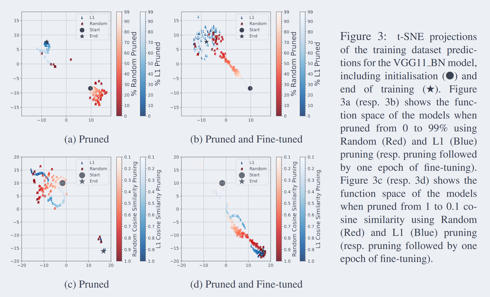
- -pruned的模型与训练后的模型在函数空间上相似, 而随机剪枝的模型与未训练的模型在函数空间上相似
- 而当我们对比余弦相似性的时候, 保持与母模型的高余弦相似性使得剪枝后的模型在函数空间上与母模型训练后的模型相似, 反之与未训练的模型相似. 这种趋势与剪枝方法无关.
- 我们假设高余弦相似度的模型之所以能在单轮微调后回归,是因为它们始终与通往局部最优的低损失"谷地"或"隧道"(Draxler等人,2018;Garipov等人,2018)保持连接,从而能够回归到相似的功能空间。我们怀疑这是因为高余弦相似度迫使网络在父函数的子空间中运行。
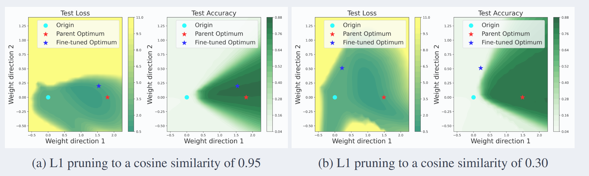
- (a) 网络在余弦相似度高时停留在局部最优的“谷地”/“通道”内,却在损失函数景观中处于功能不同的区域;这支持了Draxler等人(2018)提出的低损失流形存在的观点。
- (b) he fact that it cannot return within one epoch suggests that the network has become ‘disconnected’ from the low loss manifold
2.3. SPARSITY, LARGE PARAMETERS AND THE LOSS LANDSCAPE
We hypothesise that neural networks tend to be
- stable under increases in sparsity (e.g. through L1-pruning) but also
- inherently brittle, that is to say they are highly impacted by changes to high-magnitude parameters
- These two aspects can be quantified using the kurtosis of a network’s weight distribution: the higher the kurtosis, the more it can be pruned (see 5.4) and the more high-magnitude parameters it contains.
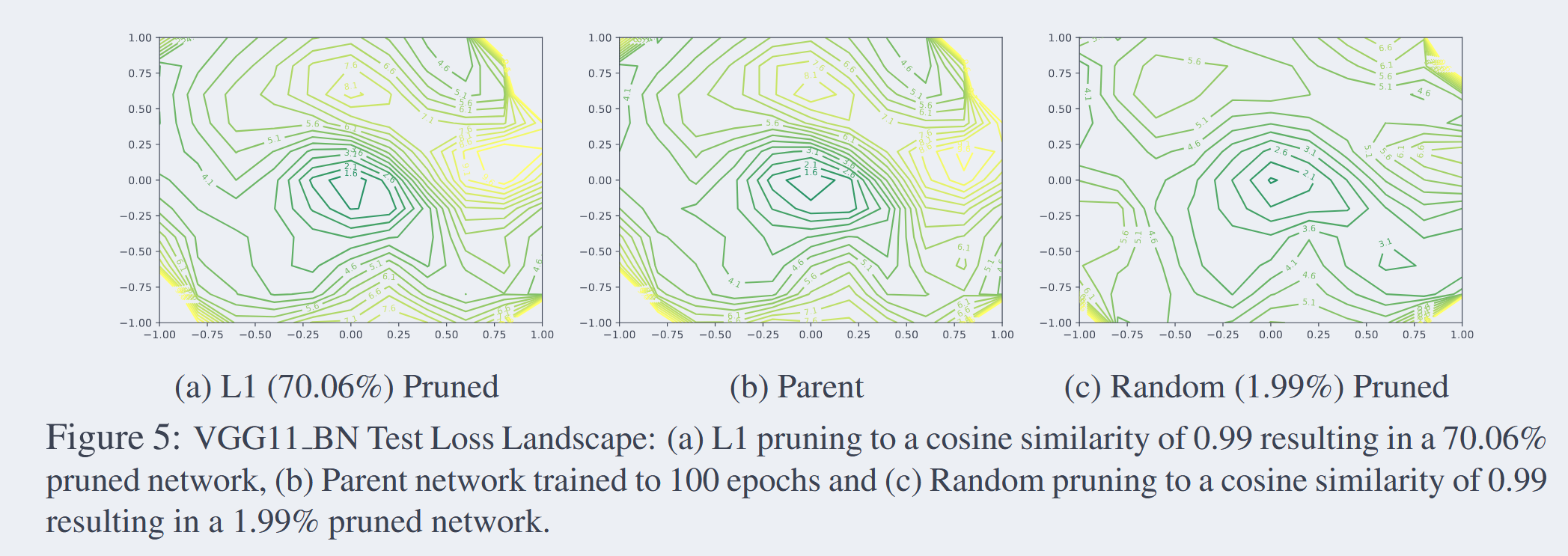
- 通过更全局地考察图5中的损失景观,我们发现剪枝方法确实会产生影响,尽管在局部父网络的小邻域内这种影响并不明显,这也解释了为何在图2c、图3c中未能显现。
- 其中L1剪掉的是幅值低的权重, 而random是均匀的机会剪到幅值高的和幅值低的权重的.
- 这些观察表明,损失函数景观很大程度上由网络中高量值参数决定。我们将这种对大型参数的敏感性称为脆弱性。
- 我们研究的模型脆性解释了为何剪枝需要与母体保持高度功能相似性:若不具备这一条件,模型将缺乏足够自由度来削弱高幅值参数的影响,因而难以探索损失函数空间的其他区域。
- 基于这一观察,我们推测在训练初期需要高参数化配置,除非获得特别优越的初始化条件。因为高参数化能提供更多的自由度,使网络更容易穿越损失函数的复杂地形——这源于网络受初始参数配置的影响更小,从而避免了因初始化不当而导致模型性能低下的情况。
2.4. OPTIMAL COSINE SIMILARITY FOR MAXIMUM MAGNITUDE PRUNING
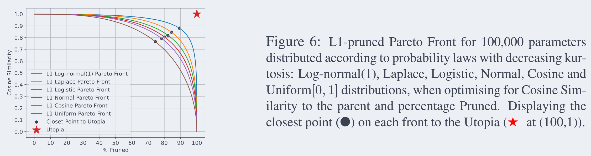
- 这一观察在直观上是合理的:具有更高峰度的分布将包含更多高幅度参数,这些参数会以相似比例同时主导公式(1)的分子与分母,从而允许在保持高余弦相似度的同时对更多低幅度权重进行L1剪枝
Summary
- 余弦相似度高的两个模型的loss landscape是相似的, 以及函数相似性(functional similarity)是相似的. 所以本文尽量尝试减小剪枝后的模型与母模型的余弦相似度的差异
- 模型的峰度高可能导致该模型在(全局)剪枝之后模型的结构可能会被大量破坏, 而导致信息流传递中断(可能有些层被剪枝过多).
Q&A
- 是否可以用峰度值作为指标来划分专家? 或者是对于不同专家峰度的峰度的层使用不同的压缩率?
takeaway
- 负对数似然: , 模型 对于第 个样本预测为真实标签 的概率值, 这个参数是越小越好的.
- 峰度
通常,我们会计算超额峰度(Excess Kurtosis),也就是将实际峰度值减去 3(正态分布的峰度值为 3),以正态分布作为基准线 0 来进行比较:
- 正态峰 / 中峰 (Mesokurtic)
- 超额峰度 = 0 (实际峰度 = 3)
- 特征:数据的分布和标准正态分布基本一致。尾部的厚度和峰的尖锐度都很“标准”。
- 尖峰厚尾 (Leptokurtic)
- 超额峰度 > 0 (实际峰度 > 3)
- 特征:与正态分布相比,它的中心更尖锐,且尾部更厚(长)。
- 意义:厚尾意味着数据集中有较多的极端值(Outliers)。在金融风险管理或处理真实世界数据时,这种分布意味着发生“黑天鹅”极端事件的概率比我们假设正态分布时要大得多。
- 平峰薄尾 (Platykurtic)
- 超额峰度 < 0 (实际峰度 < 3)
- 特征:与正态分布相比,它的峰顶更平缓,且尾部更薄(短)。
- 意义:数据往往更均匀地集中在均值附近,极端异常值非常少,结果高度可预测。